import math

import dnnlpy
import dnnlpy.nn.functional as dF
import torch
import torch.nn as nn
import torch.nn.functional as F
from torch import Tensor

print('PyTorch version:', torch.__version__)
PyTorch version: 2.14.0+cpu
上一节我们已经拆开了二维卷积的计算过程。对于输入中的每个局部窗口,卷积层会让它与卷积核逐元素相乘并求和;padding 决定输入边界如何扩展,stride 决定窗口每次移动多远,而输入通道和输出通道则决定一个卷积层需要多少组卷积核。
不过,理解公式和真正写出一个可以接收 batch、多通道输入的 Conv2d 仍然是两回事。实际的卷积层需要同时处理以下问题:
padding 和 stride 会共同决定窗口位置和输出尺寸;nn.Module 一样注册参数、初始化权重并参与反向传播。这一节我们将从一个直接的循环实现开始,逐步写出一个完整的 Conv2d 模块。这个实现不会追求运行速度,而是尽量让代码中的每一层循环都对应卷积公式中的一个维度。完成之后,我们会把它与 F.conv2d 对照,确认前向结果与梯度都一致。
import math
import dnnlpy
import dnnlpy.nn.functional as dF
import torch
import torch.nn as nn
import torch.nn.functional as F
from torch import Tensor
print('PyTorch version:', torch.__version__)PyTorch version: 2.14.0+cpu先统一这一节使用的张量布局。PyTorch 的二维卷积默认使用 NCHW 格式:
\[ X \in \mathbb{R}^{N\times C_{\text{in}}\times H\times W} \]
其中,\(N\) 是 batch size,\(C_{\text{in}}\) 是输入通道数,\(H\) 和 \(W\) 是输入的高度和宽度。
这里的“通道”可以理解为同一个空间位置上的不同信息来源。例如,一张 RGB 图像有 3 个输入通道:
\[ C_{\text{in}} = 3 \]
分别对应红色、绿色和蓝色。对于网络中间层,输入通道不再一定表示颜色,而可能表示边缘、纹理、形状等不同特征。
卷积层接收这 \(C_{\text{in}}\) 个输入通道,并生成 \(C_{\text{out}}\) 个新的输出通道:
\[ Y \in \mathbb{R}^{N\times C_{\text{out}}\times H_{\text{out}}\times W_{\text{out}}} \]
因此:
因为生成一个输出通道时,必须同时观察所有输入通道。对每个输入通道分别做局部乘加,再把结果累加起来,才得到该输出通道的一个元素。
例如:
conv = nn.Conv2d(in_channels=3, out_channels=8, kernel_size=3)表示这个卷积层:
可以粗略地把这 8 个输出通道理解为 8 张新的特征图。不同输出通道可能分别响应不同方向的边缘、颜色变化或局部纹理。
假设输入是一张 RGB 图像。一个输出特征通常不能只依赖红色通道,或者只依赖绿色通道,而需要综合观察 RGB 三个通道。因此,为了生成一个输出通道,需要为每个输入通道准备一个二维卷积核。
对于第 \(o\) 个输出通道,对应的权重为:
\[ W_o \in \mathbb{R}^{C_{\text{in}}\times K_h\times K_w} \]
它内部包含 \(C_{\text{in}}\) 个二维卷积核:
\[ \left[W_{o,0}, W_{o,1}, \ldots, W_{o,C_{\text{in}}-1} \right] \]
其中:
\[ W_{o,c}\in\mathbb{R}^{K_h\times K_w} \]
第 \(c\) 个二维卷积核只负责处理第 \(c\) 个输入通道。
如果输入有 3 个通道,那么生成一个输出通道时,需要进行 3 次二维卷积:
\[ \begin{align} X_0 \ast W_{o,0} \\ X_1 \ast W_{o,1} \\ X_2 \ast W_{o,2} \end{align} \]
然后将这 3 个结果相加:
\[ \sum_{c=0}^{C_{\text{in}}-1} X_c\ast W_{o,c} + b_o \]
这里的 \(\ast\) 表示二维卷积操作,\(b_o\) 是第 \(o\) 个输出通道对应的偏置。
因此,一个输出通道并不是由一个普通的二维卷积核生成的,而是由一组包含 \(C_{\text{in}}\) 个二维卷积核的权重共同生成的。
上面的过程只能生成一个输出通道。但卷积层通常希望提取多种不同的特征。例如,一组权重可能学习水平边缘,另一组权重可能学习垂直边缘,还有一些权重可能学习纹理或颜色变化。因此,需要准备 \(C_{\text{out}}\) 组这样的权重:
\[ W_0,W_1,\ldots,W_{C_{\text{out}}-1} \]
每一组权重都会观察全部 \(C_{\text{in}}\) 个输入通道,并生成一个输出通道。
所以,完整的卷积层权重形状是:
\[ W \in \mathbb{R}^{C_{\text{out}} \times C_{\text{in}} \times K_h \times K_w} \]
可以按照下面的方式理解这四个维度:
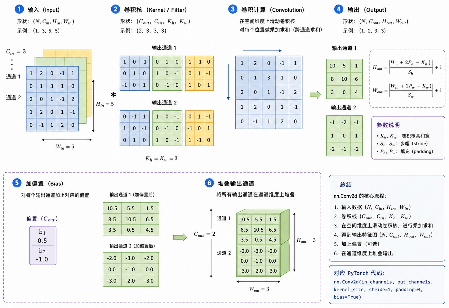
我们观察 PyTorch 中一个普通卷积层的参数形状。
conv = nn.Conv2d(
    in_channels=3,
    out_channels=8,
    kernel_size=(3, 5),
    stride=2,
    padding=(1, 2),
)

print('Weight shape:', conv.weight.shape)
print('Bias shape:', conv.bias.shape)
Weight shape: torch.Size([8, 3, 3, 5])
Bias shape: torch.Size([8])输出中的 weight 形状是 (8, 3, 3, 5),含义依次为:
(out_channels, in_channels, kernel_height, kernel_width)它表示:
因此,整个卷积层最终会生成 8 个输出通道。
nn.Conv2d 允许 kernel_size、stride 和 padding 既可以传入一个整数,也可以传入 (height, width) 二元组。例如,kernel_size=3 表示卷积核在高度和宽度方向都是 3,而 kernel_size=(3, 5) 则表示卷积核在高度方向是 3,在宽度方向是 5;stride=(2, 1) 表示卷积窗口在高度方向每次移动 2 个位置,在宽度方向每次移动 1 个位置;padding=(1, 2) 表示在输入的上下两侧各填充 1 行,在左右两侧各填充 2 列。
为了让后面的代码始终使用统一形式,我们先写一个辅助函数,把整数转换成二元组。
def as_tuple(value: int | tuple[int, int]) -> tuple[int, int]:
    """Convert an integer or a length-2 sequence to a pair."""
    if isinstance(value, int):
        return value, value

    if len(value) != 2:
        raise AssertionError('expected an integer or a sequence of length 2.')

    return tuple(map(int, value))


print('3 ->', as_tuple(3))
print('(3, 5) ->', as_tuple((3, 5)))
3 -> (3, 3)
(3, 5) -> (3, 5)接着把上一节推导过的输出尺寸写成函数。对于每个空间维度:
\[ L_{\text{out}} = \left\lfloor \frac{L_{\text{in}}+2P-K}{S} \right\rfloor + 1 \]
用代码实现一下:
def conv_output_size(
    input_size: int, kernel_size: int, padding: int, stride: int
) -> int:
    """Calculate the output size along one spatial dimension."""
    output_size = (input_size + 2 * padding - kernel_size) // stride + 1

    if output_size <= 0:
        raise RuntimeError('Calculated output size too small.')

    return output_size
这里暂时不加入 dilation,因此卷积核的有效大小就是 kernel_size 本身。Dilation 只是改变卷积核内部采样点之间的间隔,并不会改变这一节要理解的核心计算过程,可以在以后需要空洞卷积时再扩展。
现在开始实现完整的 conv2d 函数。为了让计算过程尽可能直观,我们会显式遍历:
至于输入通道和卷积核内部的求和,可以通过局部窗口与权重张量的逐元素乘法一次完成。
def conv2d_v1(
    x: Tensor,
    weight: Tensor,
    bias: Tensor | None = None,
    stride: int | tuple[int, int] = 1,
    padding: int | tuple[int, int] = 0,
) -> Tensor:
    """Apply a simple 2D convolution using explicit sliding windows."""
    if x.ndim != 4:
        raise AssertionError('Input must have shape (N, C_in, H, W).')
    if weight.ndim != 4:
        raise AssertionError('Weight must have shape (C_out, C_in, K_h, K_w).')
    if x.size(1) != weight.size(1):
        raise AssertionError('Input channels must match weight channels.')
    if bias is not None and weight.size(0) != bias.size(0):
        raise AssertionError('Bias must have shape (C_out,).')

    s_h, s_w = as_tuple(stride)
    p_h, p_w = as_tuple(padding)

    if s_h <= 0 or s_w <= 0:
        raise AssertionError('`stride` must be positive.')
    if p_h < 0 or p_w < 0:
        raise AssertionError('`padding` must be non-negative.')

    batch_size, in_channels, input_h, input_w = x.size()
    out_channels, _, k_h, k_w = weight.size()

    output_h = conv_output_size(input_h, k_h, p_h, s_h)
    output_w = conv_output_size(input_w, k_w, p_w, s_w)

    x_padded = F.pad(x, pad=(p_w, p_w, p_h, p_h))
    output = x.new_empty(batch_size, out_channels, output_h, output_w)

    for B in range(batch_size):
        for out_channel in range(out_channels):
            for i in range(output_h):
                row_start = i * s_h
                row_end = row_start + k_h

                for j in range(output_w):
                    col_start = j * s_w
                    col_end = col_start + k_w

                    window = x_padded[B, :, row_start:row_end, col_start:col_end]
                    value = torch.sum(window * weight[out_channel])

                    if bias is not None:
                        value = value + bias[out_channel]

                    output[B, out_channel, i, j] = value

    return output
虽然函数内部有四层显式循环,但每个位置上的 window 形状是:
\[ (C_{\text{in}}, K_h, K_w) \]
而 weight[out_channel] 具有完全相同的形状。两者逐元素相乘后求和,就同时完成了输入通道和卷积核空间维度上的累加。
下面用一个很小的输入观察形状变化。
x = torch.randn(2, 3, 5, 6)
weight = torch.randn(4, 3, 3, 2)
bias = torch.randn(4)

actual = conv2d_v1(x, weight, bias, stride=(2, 1), padding=(1, 0))

print('Input shape:', x.shape)
print('Weight shape:', weight.shape)
print('Output shape:', actual.shape)
Input shape: torch.Size([2, 3, 5, 6])
Weight shape: torch.Size([4, 3, 3, 2])
Output shape: torch.Size([2, 4, 3, 5])输入有 2 个样本和 3 个通道,权重包含 4 组卷积核,因此输出有 4 个通道。空间尺寸则由 kernel、padding 和 stride 共同决定。
手写实现最重要的一步不是让代码能够运行,而是确认它确实实现了预期的数学运算。我们可以把相同的输入、权重和 bias 交给 F.conv2d,然后比较两者结果。
expected = F.conv2d(x, weight, bias, stride=(2, 1), padding=(1, 0))

max_err = (actual - expected).abs().max()
print('Maximum absolute error:', max_err.item())

flag = torch.allclose(actual, expected, atol=1e-6)
print('Is the hand-written implementation close to F.conv2d?', flag)
Maximum absolute error: 1.9073486328125e-06
Is the hand-written implementation close to F.conv2d? True在浮点误差范围内,两者应该完全一致。这里的 F.conv2d 和我们手写函数做的是同一个运算,区别主要在实现方式:
因此,从零实现并不是为了在工程中替代 F.conv2d,而是为了把张量形状和卷积公式对应起来。真正使用时,仍然应该选择框架提供的高效实现。
虽然我们的实现包含切片、逐元素乘法、求和和赋值,但其中的主要数值计算仍然由 PyTorch Tensor 操作完成。因此,只要输入和参数需要梯度,autograd 就能记录计算图并计算反向传播。
我们可以分别使用手写实现和 F.conv2d 计算同一个标量损失,再比较输入、权重和 bias 的梯度。
def _copy(x: Tensor, mode: bool = True) -> Tensor:
    """Copy a tensor and set its `requires_grad` attribute."""
    return x.detach().clone().requires_grad_(mode)


x_actual = torch.randn(1, 2, 4, 5, requires_grad=True)
weight_actual = torch.randn(3, 2, 3, 2, requires_grad=True)
bias_actual = torch.randn(3, requires_grad=True)

x_expected = _copy(x_actual)
weight_expected = _copy(weight_actual)
bias_expected = _copy(bias_actual)

actual = conv2d_v1(
    x_actual,
    weight_actual,
    bias_actual,
    stride=(1, 2),
    padding=(1, 0),
)
loss_actual = actual.square().mean()
loss_actual.backward()

expected = F.conv2d(
    x_expected,
    weight_expected,
    bias_expected,
    stride=(1, 2),
    padding=(1, 0),
)
loss_expected = expected.square().mean()
loss_expected.backward()

flag = torch.allclose(x_actual.grad, x_expected.grad, atol=1e-6)
print('Is input gradient close?', flag)

flag = torch.allclose(weight_actual.grad, weight_expected.grad, atol=1e-6)
print('Is weight gradients close?', flag)

flag = torch.allclose(bias_actual.grad, bias_expected.grad, atol=1e-6)
print('Is bias gradients close?', flag)
Is input gradient close? True
Is weight gradients close? True
Is bias gradients close? True这说明我们并不需要手动推导并实现卷积的 backward。只要 forward 由可微的 PyTorch 操作组成,autograd 就可以沿着这些操作自动应用链式法则。
函数式实现接收外部传入的 weight 和 bias,但真正的卷积层需要自己持有这些可训练参数。为此,我们可以继承 nn.Module,并用 nn.Parameter 注册权重和 bias。
class Conv2d(nn.Module):
"""A minimal educational implementation of 2D convolution."""
def __init__(
self,
in_channels: int,
out_channels: int,
kernel_size: int | tuple[int, int],
stride: int | tuple[int, int] = 1,
padding: int | tuple[int, int] = 0,
bias: bool = True,
):
super().__init__()
if in_channels <= 0 or out_channels <= 0:
raise AssertionError('`in_channels` and `out_channels` must be positive.')
self.in_channels = in_channels
self.out_channels = out_channels
self.kernel_size = as_tuple(kernel_size)
self.stride = as_tuple(stride)
self.padding = as_tuple(padding)
k_h, k_w = self.kernel_size
self.weight = nn.Parameter(torch.empty(out_channels, in_channels, k_h, k_w))
if bias:
self.bias = nn.Parameter(torch.empty(out_channels))
else:
self.register_parameter('bias', None)
self.reset_parameters()
def reset_parameters(self) -> None:
nn.init.kaiming_uniform_(self.weight, a=math.sqrt(5))
if self.bias is not None:
fan_in = self.in_channels * math.prod(self.kernel_size)
bound = 1 / math.sqrt(fan_in)
nn.init.uniform_(self.bias, -bound, bound)
def forward(self, x: Tensor) -> Tensor:
return conv2d_v1(
x,
weight=self.weight,
bias=self.bias,
stride=self.stride,
padding=self.padding,
)
def extra_repr(self) -> str:
return (
f'{self.in_channels}, {self.out_channels}, '
f'kernel_size={self.kernel_size}, stride={self.stride}, '
f'padding={self.padding}, bias={self.bias is not None}'
)nn.Parameter 本质上仍然是 Tensor,但当它被赋值为 nn.Module 的属性时,PyTorch 会自动把它登记为模型参数。这样,它就会:
model.parameters() 中;state_dict() 中;.to(device) 时跟随模块移动。当不使用 bias 时,我们没有直接写 self.bias=None,而是调用:
self.register_parameter('bias', None)这样可以明确告诉 nn.Module:bias 是这个模块定义的一项参数槽位,只是当前没有实际 parameter。这也与 PyTorch 内置模块的写法保持一致。
下面实例化模块并观察它的参数。
custom_conv = Conv2d(3, 8, kernel_size=3, stride=2, padding=1)
print(custom_conv)
print('Weight shape:', custom_conv.weight.shape)
print('Bias shape:', custom_conv.bias.shape)
print('Number of parameters:', dnnlpy.count_params(custom_conv))Conv2d(3, 8, kernel_size=(3, 3), stride=(2, 2), padding=(1, 1), bias=True)
Weight shape: torch.Size([8, 3, 3, 3])
Bias shape: torch.Size([8])
Number of parameters: 224参数数量为:
\[ C_{\text{out}}C_{\text{in}}K_hK_w + C_{\text{out}} \]
其中最后一项来自 bias。如果 bias=False,就不需要最后的 \(C_{\text{out}}\) 个参数。
上面的 reset_parameters() 基本复现了 PyTorch nn.Conv2d 的默认初始化方式。卷积层的 fan_in 是一个输出元素连接到的输入数量:
\[ \text{fan\_in} = C_{\text{in}}K_hK_w \]
因为一个输出元素由所有输入通道上的 \(K_h\times K_w\) 局部窗口共同决定。
kaiming_uniform_ 会根据 fan_in 控制权重范围,避免输入经过层层线性变换后,激活值的尺度过快放大或缩小。这里为参数 a 传入 \(\sqrt{5}\),是为了与 PyTorch 线性层和卷积层的默认均匀分布边界保持一致。
Bias 的初始化范围则是:
\[ \left[-\frac{1}{\sqrt{\text{fan\_in}}}, \frac{1}{\sqrt{\text{fan\_in}}}\right] \]
reset_parameters() 不需要添加 @torch.no_grad()。nn.init 中的初始化函数本身会在不记录梯度的模式下修改参数,因此不会把初始化过程加入计算图。不过,如果我们在 reset_parameters() 中直接对叶子 Parameter 做原地赋值,就应该显式使用 torch.no_grad()。
例如,下面这种写法需要 no-grad 环境:
@torch.no_grad()
def reset_parameters(self) -> None:
self.weight.uniform_(-0.1, 0.1)而本节使用 nn.init.kaiming_uniform_ 和 nn.init.uniform_,不需要额外装饰器。
最后,把自定义模块和 nn.Conv2d 设置为完全相同的参数,比较它们的前向输出和反向梯度。
custom_conv = Conv2d(
in_channels=2,
out_channels=3,
kernel_size=(3, 2),
stride=(2, 1),
padding=(1, 0),
)
reference_conv = nn.Conv2d(
in_channels=2,
out_channels=3,
kernel_size=(3, 2),
stride=(2, 1),
padding=(1, 0),
)
with torch.no_grad():
reference_conv.weight.copy_(custom_conv.weight)
reference_conv.bias.copy_(custom_conv.bias)
actual = torch.randn(2, 2, 6, 5, requires_grad=True)
expected = _copy(actual)
actual = custom_conv(actual)
expected = reference_conv(expected)
flag = torch.allclose(actual, expected, atol=1e-6)
print('Is the hand-written Conv2d implementation close to nn.Conv2d?', flag)
loss_actual = actual.square().mean()
loss_expected = expected.square().mean()
loss_actual.backward()
loss_expected.backward()
flag = torch.allclose(actual, expected, atol=1e-6)
print('Is input gradient close?', flag)
flag = torch.allclose(custom_conv.weight.grad, reference_conv.weight.grad, atol=1e-6)
print('Is weight gradients close?', flag)
flag = torch.allclose(custom_conv.bias.grad, reference_conv.bias.grad, atol=1e-6)
print('Is bias gradients close?', flag)Is the hand-written Conv2d implementation close to nn.Conv2d? True
Is input gradient close? True
Is weight gradients close? True
Is bias gradients close? True这个测试同时验证了三件事:
因此,从数学意义上看,我们已经实现了一个最小但完整的 Conv2d。
手写版本的结构很清楚,但速度会非常慢。问题不在卷积公式本身,而在 Python 循环会逐个处理样本、通道和空间位置,无法充分利用 CPU 和 GPU 的并行计算能力。
高性能卷积通常会根据输入形状、硬件和数据类型选择不同算法。例如,一种经典思路是先把所有局部窗口重新排列成矩阵,再把卷积转换成一次大型矩阵乘法。这种方法常被称为 im2col:
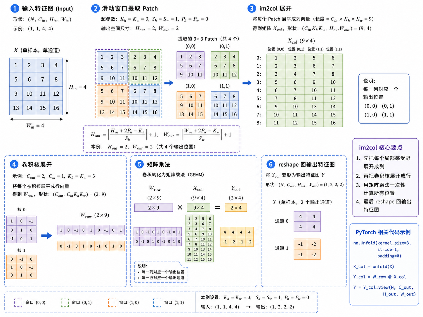
PyTorch 中的 F.unfold 就可以把二维输入的所有局部窗口展开出来。假设每个窗口包含 \(C_{\text{in}}K_hK_w\) 个元素,那么展开后的形状是:
\[ (N, C_{\text{in}}K_hK_w, H_{\text{out}}W_{\text{out}}) \]
卷积权重也可以展平为:
\[ (C_{\text{out}}, C_{\text{in}}K_hK_w) \]
两者做矩阵乘法后,再恢复空间维度,就能得到卷积输出。
下面用 F.unfold 写出同一个计算过程。这个版本已经不需要遍历每个空间位置,相比之前的版本快了很多,但它仍然主要用于解释卷积和矩阵乘法之间的关系,实际训练模型时仍然应该使用 nn.Conv2d 或 F.conv2d。
def conv2d_v2(
    x: Tensor,
    weight: Tensor,
    bias: Tensor | None = None,
    stride: int | tuple[int, int] = 1,
    padding: int | tuple[int, int] = 0,
) -> Tensor:
    """Apply 2D convolution by unfolding windows into columns."""
    if x.ndim != 4:
        raise AssertionError('Input must have shape (N, C_in, H, W).')
    if weight.ndim != 4:
        raise AssertionError('Weight must have shape (C_out, C_in, K_h, K_w).')
    if x.size(1) != weight.size(1):
        raise AssertionError('Input channels must match weight channels.')
    if bias is not None and weight.size(0) != bias.size(0):
        raise AssertionError('Bias must have shape (C_out,).')

    stride = as_tuple(stride)
    padding = as_tuple(padding)

    batch_size, in_channels, input_h, input_w = x.shape
    out_channels, _, k_h, k_w = weight.shape

    output_h = conv_output_size(input_h, k_h, padding[0], stride[0])
    output_w = conv_output_size(input_w, k_w, padding[1], stride[1])

    patches = dF.unfold(
        x,
        kernel_size=(k_h, k_w),
        padding=padding,
        stride=stride,
    )

    weight = weight.reshape(out_channels, -1)
    output = weight @ patches

    if bias is not None:
        output = output + bias.reshape(1, -1, 1)

    return output.reshape(batch_size, out_channels, output_h, output_w)
测试一下:
x = torch.randn(2, 3, 7, 6)
weight = torch.randn(5, 3, 3, 2)
bias = torch.randn(5)

actual = conv2d_v2(x, weight, bias, stride=(2, 1), padding=(1, 0))
expected = F.conv2d(x, weight, bias, stride=(2, 1), padding=(1, 0))

flag = torch.allclose(actual, expected, atol=1e-6)
print('Is the unfold implementation close to F.conv2d?', flag)
Is the unfold implementation close to F.conv2d? True当然,框架内部的实际实现远比这个例子复杂。它可能直接使用专门 kernel,也可能根据设备和输入自动选择算法。F.unfold 还会显式产生展开后的中间张量,可能消耗大量额外内存。因此,理解 F.unfold 很有帮助,但工程代码仍然应该直接使用 nn.Conv2d 或 F.conv2d。
这一节我们从卷积公式出发,实现了一个支持 batch、多输入通道、多输出通道、padding、stride 和 bias 的二维卷积函数,并进一步把它封装成了一个能够注册参数和参与训练的 nn.Module。
卷积层最重要的张量形状是:
\[ \begin{align} X&:\ (N,C_{\text{in}},H,W) \\ W&:\ (C_{\text{out}},C_{\text{in}},K_h,K_w) \\ Y&:\ (N,C_{\text{out}},H_{\text{out}},W_{\text{out}}) \end{align} \]
对于每个输出位置,卷积层取出一个形状为 \((C_{\text{in}},K_h,K_w)\) 的局部窗口,与某个输出通道对应的整组权重逐元素相乘并求和。不同空间位置共享相同的权重,而不同输出通道使用不同的权重组。
我们还验证了手写实现和 PyTorch 内置卷积在前向结果及梯度上的一致性,并通过 F.unfold 看到了卷积如何转换成矩阵乘法。循环实现适合建立直觉,展开实现适合理解计算结构,而真正训练模型时应该使用框架提供的高性能卷积 kernel。
到这里,我们已经理解并实现了 CNN 中最核心的可学习算子。但卷积层通常会保留较大的空间特征图。下一节将讨论另一类常见操作:池化与下采样。它们不负责学习新的卷积核,而是通过压缩空间尺寸,逐步扩大后续神经元能够覆盖的输入范围。