前面一节中,我们已经用 NumPy 搭好了一个可以执行 forward、backward 和 update 的两层 MLP。不过上一节使用的是随机生成的小数据,只能检查模型结构是否跑通。真正训练一个神经网络,还需要把它放到真实数据集上,重复执行很多次参数更新。
这一节我们用 MNIST 数据集训练前面实现的 MLP。为了让重点集中在神经网络本身,我们仍然使用 NumPy 手写模型、损失函数、反向传播和参数更新,不过数据集读取可以借助 torchvision 库提供的 MNIST。
本节的分工是:
TorchVision 负责帮我们拿到 MNIST 数据;
NumPy 负责完成模型训练的核心逻辑;
PyTorch Autograd 暂时不参与训练过程。
完整训练流程可以写成:
load data -> mini-batch -> forward -> loss -> backward -> update -> evaluate这正是一个监督学习训练循环的基本流程。
from collections import defaultdictimport mathimport dnnlpyimport dnnlpy.models.mlp as mlpimport matplotlib.pyplot as pltimport numpy as npimport torchvision.datasets as datasets= np.random.default_rng(42 )print ('Numpy version:' , np.__version__)
3.6.1 准备 MNIST 数据集
MNIST 是一个手写数字分类数据集。每张图片大小为 \(28 \times 28\) ,类别为 0 到 9,一共有 10 个类别。
对于 MLP 来说,我们暂时不把图像看成二维网格,而是把每张图片展平成一个长度为 784 的向量:
\[
28 \times 28 = 784
\]
也就是说,模型接收的输入形状是:
\[
X \in \mathbb{R}^{B \times 784}
\]
其中,\(B\) 是 batch size。
下载并读取 MNIST:
= dnnlpy.get_data_root()= datasets.MNIST(root, train= True , download= True )= datasets.MNIST(root, train= False , download= True )
TorchVision 读出来的图片数据存放在 data 属性中,标签存放在 targets 属性中。为了后面能够用 NumPy 训练,我们把它们转成 NumPy 数组:
= train_ds.data.numpy()= np.reshape(X_train, (- 1 , 28 * 28 ))= X_train.astype(np.float32) / 255.0 = train_ds.targets.numpy()= test_ds.data.numpy()= np.reshape(X_test, (- 1 , 28 * 28 ))= X_test.astype(np.float32) / 255.0 = test_ds.targets.numpy()print ('X_train shape:' , X_train.shape)print ('y_train shape:' , y_train.shape)print ('X_test shape:' , X_test.shape)print ('y_test shape:' , y_test.shape)
X_train shape: (60000, 784)
y_train shape: (60000,)
X_test shape: (10000, 784)
y_test shape: (10000,)
这里做了两件事:
使用 reshape(-1, 28 * 28) 把每张图片展平成 784 维向量;
除以 255.0,把像素值从 \([0, 255]\) 缩放到 \([0, 1]\) 。
这种归一化虽然简单,但对训练很有帮助。因为如果输入值过大,线性层输出的 logits 也可能变得很大,训练会更不稳定。
我们可以看几张图片:
= plt.figure(1 , figsize= (8 , 2 ))= fig.subplots(1 , 6 )for i, ax in enumerate (axes.ravel()):28 , 28 ), cmap= 'gray' )'off' )f'label: { y_train[i]} ' , fontsize= 10 )'highdpi' )
注意,虽然我们把图片展平成了向量,但这只是为了适配 MLP 的输入。原始图像仍然是二维的,只是 MLP 不显式利用这种空间结构。后面我们讲 CNN 会重新引入空间结构的概念。
3.6.2 Mini-batch 数据迭代
训练神经网络时,我们通常不会一次性把所有训练数据都送进模型,而是把数据分成很多 mini-batch。
如果 batch size 为 \(B\) ,那么一次训练步骤只使用:
\[
X_{\text{batch}} \in \mathbb{R}^{B \times 784}
\]
和对应标签:
\[
y_{\text{batch}} \in \mathbb{R}^{B}
\]
这样做有几个好处:
每次更新的计算量更小;
梯度带有一定随机性,有助于训练;
更接近实际深度学习框架中的训练方式。
我们先写一个简单的 mini-batch 迭代器:
class DataLoader:def __init__ (self ,int ,bool = True ,self .X = Xself .y = yself .batch_size = batch_sizeself .shuffle = shuffledef __iter__ (self ):= np.arange(len (self .X))if self .shuffle:for start in range (0 , len (self .X), self .batch_size):= indices[start : start + self .batch_size]yield self .X[idx], self .y[idx]def __len__ (self ):return math.ceil(len (self .X) / self .batch_size)
每个 epoch 开始时,我们会打乱训练集顺序。这样模型不会每一轮都按照完全相同的样本顺序学习。
3.6.3 计算 Accuracy
分类任务中,除了 loss,我们还经常关心 accuracy。
模型输出的是 logits:
\[
Z \in \mathbb{R}^{B \times 10}
\]
每一行对应一张图片在 \(10\) 个类别上的分数。预测类别就是分数最大的那个类别:
\[
\hat{y}_i = \arg\max_j Z_{i,j}
\]
对应的 NumPy 实现是:
def accuracy(logits: np.ndarray, labels: np.ndarray) -> float := np.argmax(logits, axis= 1 )= np.sum (pred == labels)return correct / len (labels)
我们这里直接使用 np.argmax 来得到预测类别,然后和真实标签比较,计算正确率。注意,虽然 softmax 可以把 logits 转成概率,但它不会改变 logits 的大小顺序,所以我们直接在 logits 上使用 np.argmax 就可以了。
3.6.4 训练循环
现在我们有了 Mini-batch 迭代器和评估函数,再加上前面实现的模型、损失函数和优化器,我们就有了训练神经网络的所有组件,接下来就可以写完整训练循环了。
先把数据加载器、模型、损失函数和优化器都准备好:
= DataLoader(X_train, y_train, batch_size= 128 , shuffle= True )= DataLoader(X_test, y_test, batch_size= 128 , shuffle= False )= mlp.MLP(input_dim= 784 , hidden_dim= 256 , num_classes= 10 )= mlp.CrossEntropyLoss()= mlp.SGD(model.parameters(), lr= 0.1 )= defaultdict(list )
每个 mini-batch 的训练步骤是:
forward -> loss -> backward -> update完整训练代码如下:
= 10 for epoch in range (1 , num_epochs + 1 ):= 0.0 = 0 for X, y in train_dl:= model(X)= loss_fn(logits, y)= loss_fn.backward()= model.backward(dlogits)+= loss.item()+= np.sum (np.argmax(logits, axis= 1 ) == y)= train_loss / len (train_dl)= correct_samples / len (train_ds)'loss' ].append(avg_train_loss)'acc' ].append(avg_train_acc)= 0.0 = 0 for X, y in test_dl:= model(X)= loss_fn(logits, y)+= loss.item()+= np.sum (np.argmax(logits, axis= 1 ) == y)= test_loss / len (test_dl)= correct_samples / len (test_ds)'test_loss' ].append(avg_test_loss)'test_acc' ].append(avg_test_acc)= len (str (num_epochs))print (f'Epoch [ { epoch: {n}d} / { num_epochs: {n}d} ] ' f'| loss: { avg_train_loss:.4f} ' f'| acc: { avg_train_acc:.4f} ' f'| test_loss: { avg_test_loss:.4f} ' f'| test_acc: { avg_test_acc:.4f} '
Epoch [ 1/10] | loss: 0.4410 | acc: 0.8816 | test_loss: 0.2687 | test_acc: 0.9252
Epoch [ 2/10] | loss: 0.2447 | acc: 0.9310 | test_loss: 0.2067 | test_acc: 0.9398
Epoch [ 3/10] | loss: 0.1948 | acc: 0.9455 | test_loss: 0.1753 | test_acc: 0.9478
Epoch [ 4/10] | loss: 0.1635 | acc: 0.9541 | test_loss: 0.1476 | test_acc: 0.9564
Epoch [ 5/10] | loss: 0.1409 | acc: 0.9605 | test_loss: 0.1332 | test_acc: 0.9601
Epoch [ 6/10] | loss: 0.1234 | acc: 0.9655 | test_loss: 0.1212 | test_acc: 0.9651
Epoch [ 7/10] | loss: 0.1101 | acc: 0.9699 | test_loss: 0.1130 | test_acc: 0.9665
Epoch [ 8/10] | loss: 0.0993 | acc: 0.9730 | test_loss: 0.1040 | test_acc: 0.9687
Epoch [ 9/10] | loss: 0.0902 | acc: 0.9755 | test_loss: 0.0974 | test_acc: 0.9713
Epoch [10/10] | loss: 0.0830 | acc: 0.9775 | test_loss: 0.0928 | test_acc: 0.9730
这段代码虽然不长,但已经包含了训练神经网络的核心逻辑。
对于每个 mini-batch:
model(X) 计算 logits;loss_fn(logits, y_batch) 计算 loss;loss_fn.backward() 得到关于 logits 的梯度;model.backward(dlogits) 把梯度传回每个参数;optimizer.step() 根据梯度更新参数。
也就是说,我们实现了 PyTorch 训练循环中最核心的部分。
3.6.5 观察训练曲线
训练完成后,我们可以把 loss 和 accuracy 画出来。
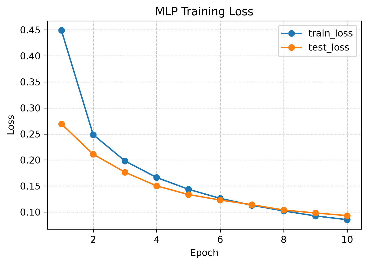
先看训练集和测试集的 loss:
= plt.figure(2 , figsize= (6 , 4 ))= fig.add_subplot(1 , 1 , 1 )= np.arange(1 , num_epochs + 1 )'loss' ], marker= 'o' )'test_loss' ], marker= 'o' )= '--' , alpha= 0.7 )'Epoch' )'Loss' )'train_loss' , 'test_loss' ])'MLP Training Loss' )
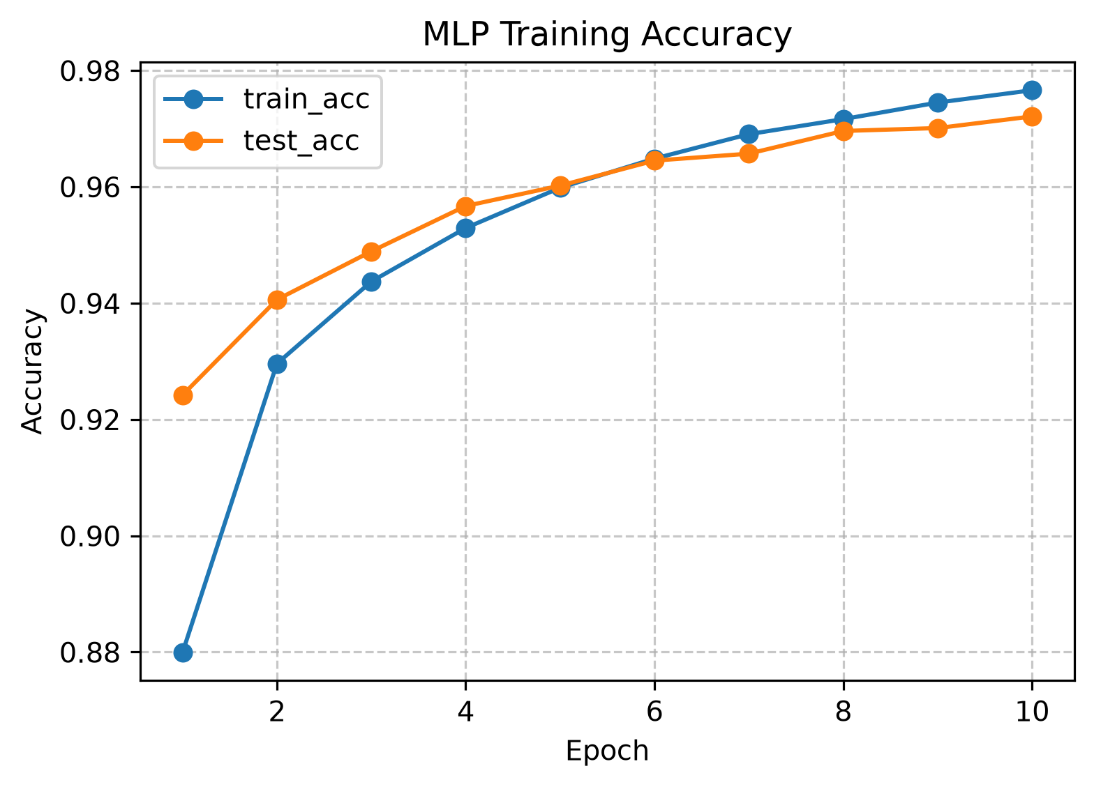
再看训练集和测试集的准确率:
= plt.figure(2 , figsize= (6 , 4 ))= fig.add_subplot(1 , 1 , 1 )= np.arange(1 , num_epochs + 1 )'acc' ], marker= 'o' )'test_acc' ], marker= 'o' )= '--' , alpha= 0.7 )'Epoch' )'Accuracy' )'train_acc' , 'test_acc' ])'MLP Training Accuracy' )
如果训练正常,我们通常会看到:
Training loss 逐渐下降;
Training accuracy 逐渐上升;
Testing accuracy 也逐渐上升,但不一定和 training accuracy 完全一样。
这说明模型确实通过梯度下降学到了某些能区分数字的模式。
3.6.6 查看预测结果
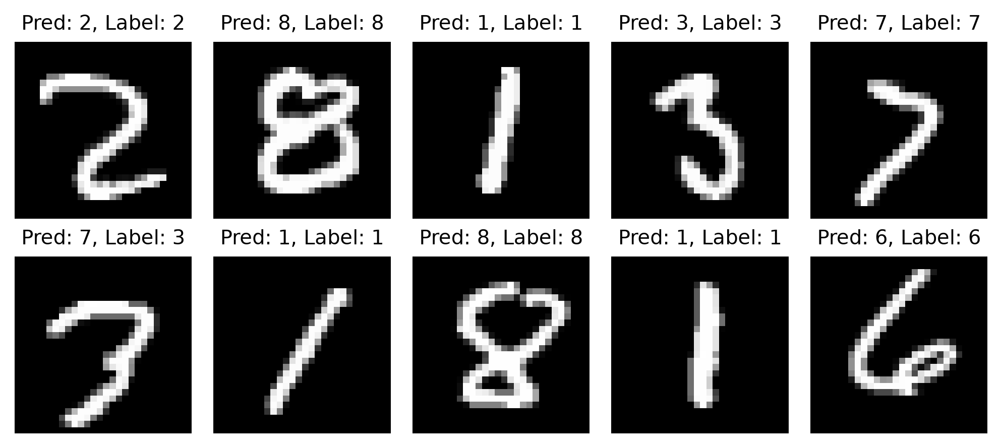
最后,我们可以随机挑几张测试图片,看看模型的预测结果。
= rng.choice(len (X_test), size= 10 , replace= False )= X_test[indices]= y_test[indices]= model(x_samples)= np.argmax(logits, axis= 1 )
可视化这些样本:
= plt.figure(3 , figsize= (7 , 3.2 ))= fig.subplots(2 , 5 )for i, ax in enumerate (axes.ravel()):28 , 28 ), cmap= 'gray' )'off' )f'Pred: { y_preds[i]} , Label: { y_samples[i]} ' , fontsize= 10 )
如果预测正确,pred 和 label 会相同;如果预测错误,也可以观察一下模型到底把这个数字认成了什么。
这一步不是训练必须的,但它很有用,因为它可以帮助我们直观地理解模型的表现,看看它在哪些样本上做得好,哪些样本上做得不好。这样,我们就可以进一步分析模型的局限性,或者思考如何改进模型。
3.6.7 MLP 在图像任务上的局限
到这里,我们已经用 NumPy 手写了一个可以在 MNIST 上训练的 MLP。不过,MLP 处理图像有一个明显问题:它把 \(28 \times 28\) 的二维图片直接展平成 784 维向量。这样做虽然简单,但会丢掉图像中的空间结构。
例如,在原图中相邻的两个像素,展平之后仍然可能相邻;但模型本身并不知道它们来自二维网格中的相邻位置。对于 MLP 来说,输入只是一个普通向量:
\[
X = [x_1, x_2, \dots, x_{784}]
\]
它不会显式利用局部区域、平移结构或二维邻域关系。
这也是为什么后面处理图像时,我们通常会引入更适合图像结构的模型,例如卷积神经网络(CNN)和 Vision Transformer(ViT)。不过,在理解神经网络训练机制时,MLP 仍然是最好的起点之一。因为它已经包含了深度学习训练的核心组件:
可学习参数;
前向传播;
损失函数;
反向传播;
梯度下降更新;
训练集和测试集评估。
3.6.8 本章小结
这一节我们把前面实现的 NumPy MLP 放到了 MNIST 数据集上,完成了一个完整的训练实验。
我们先使用 torchvision.datasets.MNIST 读取数据,再把图像展平成 784 维向量,并归一化到 \([0, 1]\) 。随后,我们手写了 mini-batch 迭代器、accuracy 计算函数和训练循环。
每个 mini-batch 的训练步骤都是:
forward -> loss -> backward -> update对应到代码中,就是:
# forward = model(x)= loss_fn(logits, y)# backward = criterion.backward()# update 这个过程没有使用 PyTorch Autograd,所有梯度都来自我们前面推导并实现的反向传播公式。但是,这就产生了一个问题:
如果我们计算的梯度错了怎么办?
下一节我们会讨论一个很实用的梯度检查方法:数值梯度检查。