Previously, we have already seen several types of generative models. GAN is like an adversarial game, letting the generator produce realistic samples in one step; AutoEncoder learns compression and reconstruction; VAE starts to explicitly model probability distributions and can sample from latent variables; and when it comes to Diffusion Model, its idea is quite different again:
It does not draw the image in one step, but starts from a ball of noise and washes the image out little by little.
This may sound a bit strange the first time you hear it: denoising, isn’t it just making a dirty image clean? What does this have to do with generation? Why can we start from pure noise, denoise repeatedly, and finally get a real image?
In this section, we will not rush into the complete derivation first, but first explain this core intuition clearly. You will see that the starting point of DDPM is actually very simple: if one-step generation is too difficult, then split it into many simple small steps.
import randomimport dnnlpyimport matplotlib.pyplot as pltimport torchimport torchvision.datasets as datasetsimport torchvision.transforms.v2 as v2plt.rc('figure', dpi=100)dnnlpy.set_matplotlib_format('highdpi')print('PyTorch version:', torch.__version__)
PyTorch version: 2.12.1+cpu
14.1.1 Generation: The Reverse Process of Adding Noise
Let’s first think about a very simple process. Suppose we have a real image \(x_0\). Now we continuously add a little bit of Gaussian noise to it:
In the first step, add a little, and the image becomes a little blurry;
In the second step, add a little more, and there are fewer details;
In the third step, add a little more, and even the contours start to disappear;
…
After adding for many, many steps, it will eventually become an almost pure Gaussian noise image.
This tells us one thing: between the real data distribution and the Gaussian noise distribution, maybe they can be connected through many very small changes. Then, since we can slowly push a real image toward the noise side, a natural idea is:
Can we do it in reverse?
That is, can we start from pure noise, make only a small correction at each step, and finally slowly walk back to the real image distribution?
This is the most core idea of DDPM.
Below, we first do not train any model. We just take one image and do a simple thing: every few steps, add some Gaussian noise to it, and gradually increase the noise level. Let’s look at how the image gradually loses its structure.
From the figure above, we can find that when the noise is small, the general structure of the image is still there; when the noise gradually increases, the model needs to recover more and more information; when the noise becomes large enough, the image almost only has random pixels left.
So, going from a clear image to pure noise is not completed with a snap, but can be divided into many small steps. Then in reverse, from noise back to image, is it also possible to divide it into many small steps? In other words, we are completing a reverse process of adding noise. Then, why do we add noise step by step, instead of doing it all at once?
14.1.2 Why Is Step by Step Easy, While One Step Is Hard?
Suppose now you are asked to do two tasks.
Task A: generate a cat image in one step
The input is a ball of random noise, and the output is directly a complete, natural, structurally reasonable, and detail-rich cat image.
This is very hard. Because the model has to decide many things at once: what is the cat’s pose? Which direction is the face pointing? What is the background? How should the fur texture be drawn? How should the lighting be arranged? Is the overall structure natural? That is to say, one-step generation is essentially learning a very complex global mapping. So this task is very difficult for the model.
Task B: give you an image with a little noise, and ask you to remove the noise a little
This task is much simpler. Because at this time, part of the structure has already been preserved in the image, the rough contour is still there, the local shapes are still there, and the noise is just covering these structures. Just like the experiment above, even if 100% noise is added, we can still roughly distinguish the digit in the image. The model is the same. At this time, the model does not need to create everything from scratch. It only needs to know, in this image, which parts are more like noise? In which direction should it be corrected a little? This is much easier than generating the whole image in one step.
Therefore, the core strategy of Diffusion Model is: do not force the model to learn to generate an image directly from random numbers in one go, but split this hard problem into many simple small problems, and remove only a little noise at each step. This is very similar to a common idea in deep learning: if a complex mapping is split into many simple mappings, it is often easier to learn.
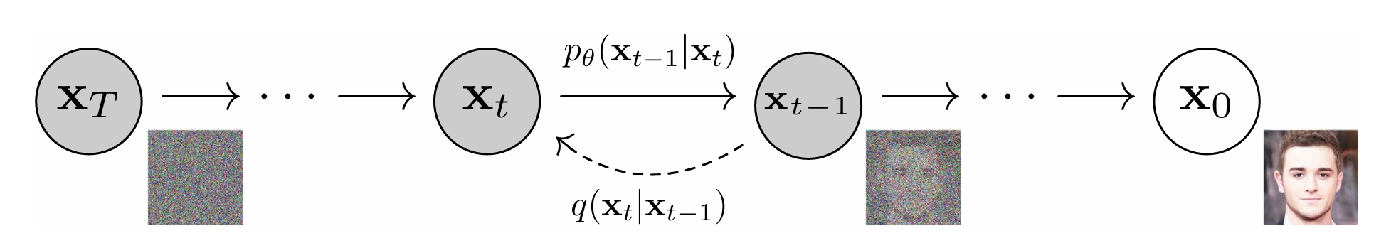
14.1.3 The Core Idea of DDPM: First Learn Destruction, Then Learn Recovery
DDPM actually does two things.
First step: design a forward noising process
We manually specify a simple and fixed process, adding noise to the real image step by step until it finally becomes standard Gaussian noise:
Here, \(x_0\) is the real image; \(x_t\) is the result after adding noise at step \(t\); \(x_T\) is basically pure noise.
This process does not need learning. It is defined by ourselves. Its role is to gradually turn a complex data distribution into a Gaussian distribution that we are very familiar with and very easy to sample from.
Second step: learn a reverse denoising process
Since the forward process turns the image into noise, we train a neural network to learn the process in the reverse direction:
That is, input the current noisy image, predict how much noise should be removed in this step, and get an image that is slightly cleaner; repeat this many times, and finally get a clear image.
Then, when we want to generate an image, it is very simple: start from random Gaussian noise, repeatedly call the denoising network, and finally generate a sample. So, DDPM’s generation is not direct generation like GAN, but starts from noise and denoises gradually.
Figure 14.1.3: Schematic diagram of the DDPM generation process (Ho et al. 2020, fig. 2)
Intuitively, we already feel that this makes sense. From the perspective of probabilistic modeling, it is actually also very natural.
We know that no matter what kind of generative model it is, what it ultimately wants to learn is the data distribution \(p_{\text{data}}(x)\). Traditional generative models directly or indirectly approximate this distribution, while DDPM first manually defines a forward process, slowly turning the data distribution into a Gaussian distribution; then it learns its reverse process, letting the model learn how to go from the Gaussian distribution back to the data distribution.
That is, it does not directly force itself to learn:
Each step only makes a small modification, so the learning difficulty is lower and it is more stable.
So, DDPM successfully turns an image generation problem into a denoising problem. We first manually make the image worse (adding noise), and then teach the network how to make the image better (denoising). This is its core idea. The output of the network at each step is how much noise we should remove from the image in this step.
14.1.4 The Training Objective of DDPM: Guess the Noise
In the most common DDPM notation, we write the noisy sample at step \(t\) as:
There is no need to fully understand this formula right now. We only need to first grasp what it expresses:
Part of the original image \(x_0\) is still kept;
Part of the Gaussian noise \(\epsilon\) is added;
As \(t\) increases, the noise part becomes stronger and stronger;
When \(t\) is large enough, \(x_t\) becomes closer and closer to pure noise.
Here, \(\bar{\alpha}_t\) is a coefficient that changes over time, controlling the ratio between the original image and the noise. It monotonically decreases over time, so as \(t\) increases, the original image component gradually decreases and the noise component gradually increases. We will talk about its specific form later. For now, do not rush.
During training, the model’s task is usually:
\[
\epsilon_\theta(x_t, t) \approx \epsilon
\]
That is, give it a noisy image at some time, and let it guess the noise mixed into it. This is why in many DDPM papers and code implementations, the final loss function looks like a very simple mean squared error:
On the surface, it is only guessing noise, but in essence, it is learning how to slowly pull the sample from the noise direction back to the data distribution.
14.1.5 Summary
Now we can summarize the overall process of DDPM.
Training stage
During training, we take a real image \(x_0\), randomly choose a time step \(t\), and then:
According to the predefined rule, add noise of the corresponding strength to it and get \(x_t\);
Input \(x_t\) and the time step \(t\) into the neural network;
Let the network predict the noise added in this step;
Use the predicted noise and the real noise to compute the loss and train the network.
So the essence of training is to let the model learn to identify and estimate noise under any noise level.
Generation stage
During generation, we no longer input a real image, but directly start from pure Gaussian noise \(x_T\):
Input Gaussian noise;
The network predicts the noise in it;
Remove a little noise and get a cleaner image;
Repeat this, walking from \(T\) to \(0\).
The final \(x_0\) is the generated sample we want.
The essence of DDPM can be understood in three sentences:
First add noise to real data step by step until it reaches a Gaussian distribution;
Then train the model to learn the reverse process of this process;
Therefore, during generation, as long as we start from Gaussian noise and walk back in reverse, we can get samples.
Overall, the idea of DDPM is that if the complex generation task is too hard, then split it into many simple small tasks. Of course, although the core idea of DDPM is very simple, its mathematical derivation and detailed design are still very headache-inducing. Later, we will slowly unfold and discuss them.
In the next section, we will formally enter the mathematical form and look at how DDPM’s forward noising and reverse denoising are defined, as well as the relationship between them. In the end, you will find that DDPM’s training objective and generation process are both derived from a very natural probabilistic modeling perspective, rather than being designed arbitrarily.