15.1 CLIP: Mapping Images and Text into the Same Semantic Space
Author
jshn9515
Published
2026-04-07
Modified
2026-04-07
In the previous chapters, we have seen many vision and text models. Whether for classification, detection, or generation, most of these models only process one modality, that is, the image or the text itself. But if we take one step back, the supervision signals in the real world are not always neat category labels. More often, what we get is an image paired with a natural language description, such as “this is a cat lying on a sofa”, “a blue car parked by the road”, or “a person surfing by the sea”.
Then, a natural question is:
Can we directly use the correspondence between images and text to train a model?
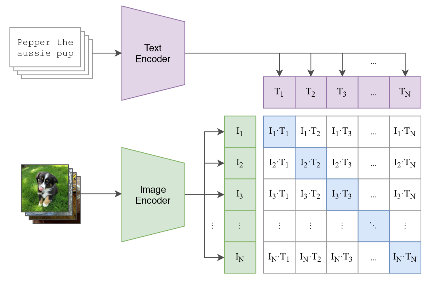
CLIP (Contrastive Language-Image Pretraining) (Radford et al. 2021) gives the answer: yes. Its core idea is very direct: let the model look at images and text at the same time, and learn which image should be closer to which sentence, and which image should not be close to which sentence. If this objective is learned well enough, then the model will eventually map both images and text into the same semantic space. As a result, tasks such as image classification, image-text retrieval, and zero-shot recognition can all be unified into a problem of computing similarity.
In this section, we will make the core idea of CLIP clear. You will see that it does not explicitly train a traditional classifier, but puts the supervision signal on image-text alignment. It is exactly because of this that it has strong zero-shot learning ability.
import osimport randomimport dnnlpyimport IPython.display as ipyimport matplotlib.pyplot as pltimport PIL.Image as Imageimport seaborn as snsimport torchimport torch.nn.functional as Fimport torchvision.datasets as datasetsimport transformersfrom torch import Tensorfrom transformers import CLIPModel, CLIPProcessorplt.rc('figure', dpi=100)print('PyTorch version:', torch.__version__)print('Transformers version:', transformers.__version__)
15.1.1 Why Put Images and Text Together for Learning?
Traditional image classification usually relies on manually annotated discrete categories, such as “cat”, “dog”, and “car”. This kind of supervision is certainly effective, but it also has two obvious limitations.
First, the category set is fixed. If the model has only seen 1000 categories, then it is naturally restricted to these 1000 categories. Even if an image expresses “a dog catching a frisbee” or “two people cooking in a kitchen”, a traditional classifier usually can only give static categories such as “dog” or “person”, and it is hard to directly use these more complete semantic descriptions.
Second, manual annotation is expensive. You need to first define a label system, and then ask annotators to label images one by one. But on the Internet, there naturally exist a large number of image-text pairs, such as webpage images and titles, product images and descriptions, and social media images and captions. These data have some noise, but their scale is extremely large.
So, a very attractive idea appears:
Do not compress the supervision signal into fixed categories, but directly use natural language itself as supervision.
The benefit of doing this is obvious. Natural language itself carries rich semantics. It can represent not only categories, but also attributes, relations, actions, and scenes. For example, “a tabby cat running on the grass” carries much more information than a single “cat” label.
From this perspective, CLIP’s training objective is actually very intuitive: given a batch of images and a batch of texts, let the model judge which image and which sentence form a pair.
It looks like it is doing matching, but what this task really requires the model to learn is: what is in the image, what the text is saying, and whether the two are semantically consistent. To complete this task, the model cannot only memorize fixed categories. Instead, it must map image semantics and text semantics into a space where they can be directly compared. It is exactly because of this that what CLIP learns is a kind of cross-modal semantic alignment.
This training method also has a very important result: the model is no longer strictly limited by a fixed label table. During inference, we may not even need to retrain a new classification head. As long as we write some text descriptions, we can directly match the image with these texts. In other words, during training, we use text to supervise the model; during testing, we can also directly write a set of text descriptions and let the model judge which sentence best matches the image.
This is also why CLIP looks like it is learning “matching”, but finally shows more flexible ability than traditional classification with fixed labels.
15.1.2 CLIP’s Core Structure: Two Encoders + a Similarity Matrix
CLIP’s structure can be summarized into two parts.
An image encoder \(f_\theta(\cdot)\), which encodes images into vectors (for example, ResNet or ViT);
A text encoder \(g_\phi(\cdot)\), which encodes text into vectors (for example, Transformer).
In practice, CLIP does not directly send this cosine similarity into the following softmax. Instead, it first multiplies it by a learnable scaling coefficient \(\tau\):
\[
s_{ij} = \tau \cdot \cos(\theta_{ij})
\]
This \(\tau\) can be understood as a knob that enlarges the score gap. It does not change which image-text pair is more similar, but it changes the degree to which these similarity scores are separated. The larger \(\tau\) is, the more prominent the best-matching image-text pair becomes, the lower the scores of wrong pairs are pushed, and the sharper the distribution after softmax becomes; the smaller \(\tau\) is, the closer the scores are, and the model’s judgment will look less decisive.
Some materials write it in the form of temperature \(T\):
These two ways of writing are essentially the same, only with different notation, where \(\tau = \frac{1}{T}\).
The temperature here is somewhat similar in mathematical effect to the temperature in generative models: both affect how sharp the softmax distribution is. However, in generation tasks such as LLMs, temperature is often informally understood as “controlling creativity” or “controlling divergence”, because it further affects randomness during sampling; while in CLIP, it does not control generation, but is used to adjust the scale of image-text matching scores, making the difference between positive and negative samples more obvious. In other words, temperature in generative models more often affects “what will be generated”, while temperature in CLIP more often affects “who the model sees as more similar”.
Note
For intuition, above we directly wrote it as cosine similarity. In actual implementation, usually we do not separately call cosine similarity. Instead, we first apply L2 normalization to image features and text features, and then compute their dot product. Because the dot product after normalization is exactly equal to cosine similarity mathematically, these two ways of writing are essentially the same. The benefit of writing it this way is that it is more convenient to construct the similarity matrix of the whole batch later.
After we have the similarity score \(s_{ij}\) for a single image-text pair, we can pair every image and every text in a batch, and get a similarity matrix:
In this way, every image can compute similarity once with every text in the batch, and every text can also compute similarity once with every image in the batch. If the \(i\)-th image and the \(i\)-th text are a pair, then we want the scores on the diagonal of the matrix to be as large as possible, and the scores off the diagonal to be as small as possible. That is:
Positive pairs should be as close as possible;
Negative pairs should be as far away as possible.
This is CLIP’s core training signal.
In code, we directly load a pretrained CLIP model, get its image encoder and text encoder, and then send a batch of images and a batch of texts into it to get their feature vectors. Next, we apply L2 normalization to these feature vectors, compute their dot product, and multiply by the scaling coefficient \(\tau\). Then we obtain the similarity matrix \(S\).
# 1) load pretrained CLIP model and processormodel_id ='openai/clip-vit-base-patch32'model = CLIPModel.from_pretrained(model_id, device_map=device)processor = CLIPProcessor.from_pretrained(model_id, device_map=device)model.eval()ipy.clear_output()
# 2) Prepare a batch of imageslabels = ['dog', 'cat', 'car', 'pizza']file_paths = [os.path.join('figures', f'ch15-{label}.png') for label in labels]images = [Image.open(fp).convert('RGB') for fp in file_paths]# 3) Prepare a batch of text promptstexts = [f'a photo of a {label}'for label in labels]# 4) Extract features and compute similarity matrixwith torch.inference_mode(): image_input = processor(images=images, return_tensors='pt').to(device) text_input = processor(text=texts, padding=True, return_tensors='pt').to(device)# Both image_features and text_features have shape (batch_size, feature_dim) image_features = model.get_image_features(**image_input).pooler_output text_features = model.get_text_features(**text_input).pooler_output image_features = F.normalize(image_features, dim=-1) text_features = F.normalize(text_features, dim=-1) similarity = model.logit_scale.exp() * image_features @ text_features.Tfig = plt.figure(1, figsize=(4, 3))ax = fig.add_subplot(1, 1, 1)sns.heatmap( similarity.cpu(), annot=True, fmt='.2f', cmap='Blues', linewidths=0.5, xticklabels=labels, yticklabels=labels, ax=ax,)ax.set_xlabel('text')ax.set_ylabel('image')ax.set_title('CLIP similarity matrix')dnnlpy.set_matplotlib_format('svg')plt.show()
This similarity matrix explains very well how CLIP works: it pulls correctly paired images and text closer. From the figure, we can see that the highest score in each row appears on the diagonal. For example, the dog image has the highest score with the dog text, and the cat image has the highest score with the cat text. This shows that the model can basically judge which text this image is most like.
At the same time, this matrix also shows that what CLIP learns is not only “right” or “wrong”. For example, although dog and cat are not completely matched, the score between them is still relatively high, because dogs and cats are semantically close in the first place, both belonging to “animals”; while pizza is far away from animals, so the score is lower. In other words, CLIP learns a semantic feeling of “who is more like whom”, rather than simply separating every category rigidly.
15.1.3 CLIP’s Training Objective: Bidirectional Contrastive Learning
Suppose there are \(N\) image-text pairs in a batch, and the \(i\)-th image corresponds to the \(i\)-th text. Then, for the \(i\)-th image, we can treat the \(i\)-th text as the correct category, and treat the other \(N-1\) texts as negative classes. So, the image-to-text loss can be written as:
This objective looks very similar to classification, but it is different from ordinary classification. The categories here are not fixed labels, but the paired samples in the current batch. In other words, CLIP is not learning a classifier with fixed categories, but learning a cross-modal similarity space.
CLIP loss: 0.7495301365852356
image -> text predictions: [0, 1, 2, 3]
text -> image predictions: [0, 1, 2, 3]
From the code, you can see that the implementation of CLIP loss is actually very concise. As long as you have obtained image features and text features, the training objective after that is almost a bidirectional cross-entropy, plus a scaling coefficient.
This is also one of the beautiful parts of CLIP: the model architecture is not complicated. The key is that the scale of training data and the supervision method have changed. It does not rely on fine-grained category labels, but relies on massive image-text paired data, letting images and language naturally align in the same space.
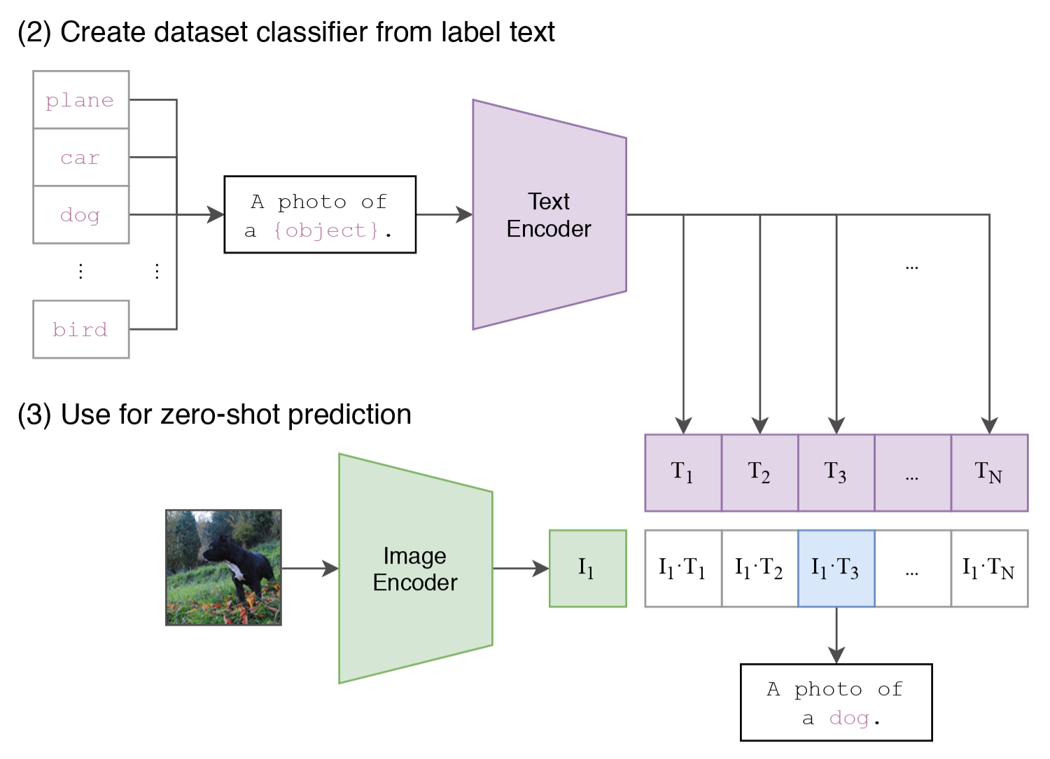
15.1.4 Why Can CLIP Do Zero-Shot Classification?
Before discussing this question, let’s first talk about what zero-shot classification is.
Simply put, zero-shot classification refers to the ability of a model to still correctly recognize a category when it has not seen training samples of that category. For traditional classifiers, this is almost impossible, because their last layer is a linear layer with a fixed number of categories, and the model can only output probabilities for these predefined categories. So once the category table changes, you often need to retrain or fine-tune the model.
But CLIP is different. What it outputs is not fixed category probabilities, but an image vector and a text vector. Therefore, when you want to do classification, you only need to write the candidate categories as several prompts, for example:
“a photo of a cat”
“a photo of a dog”
“a photo of a truck”
Then encode these texts into vectors as well, and compute their similarity with the image vector. Whichever prompt is the closest, the image is assigned to that category.
That is to say, CLIP does not use a fixed linear layer to output categories like traditional classification models. Instead, during inference, it uses a group of text descriptions to generate the corresponding category vectors, and then makes the judgment according to the similarity between the image and these vectors. This is the root of zero-shot:
Categories are defined by language during inference, rather than hard-coded during training.
Of course, there is also a very important practical detail here. The text encoder of the original OpenAI CLIP was mainly trained on English data, so in many cases English prompts work obviously better than Chinese prompts. This is not a limitation of the CLIP theory itself, but a result of the training corpus distribution.
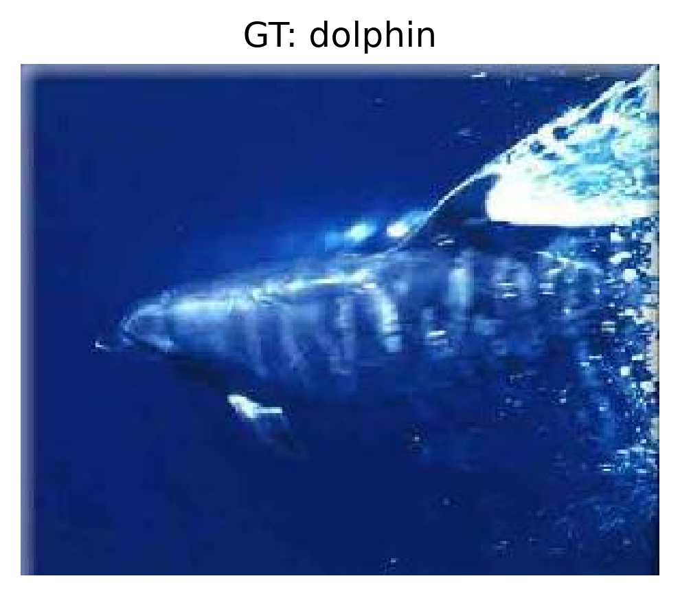
root = dnnlpy.get_data_root()dataset = datasets.Caltech101(root, target_type='category', download=True)idx = random.randrange(len(dataset))image, label = dataset[idx]prompts = [f'a photo of a {name}'for name in dataset.categories]inputs = processor(image, prompts, padding=True, return_tensors='pt').to(device)with torch.inference_mode(): outputs = model(**inputs) probs = outputs.logits_per_image.softmax(dim=-1)[0]topk = probs.topk(5)pred_names = [dataset.categories[i] for i in topk.indices.tolist()]pred_scores = topk.values.tolist()fig = plt.figure(2, figsize=(4, 4))ax = fig.add_subplot(1, 1, 1)ax.imshow(image)ax.axis('off')ax.set_title(f'GT: {dataset.categories[label]}')dnnlpy.set_matplotlib_format('highdpi')plt.show()z =zip(pred_names, pred_scores, strict=True)for rank, (name, score) inenumerate(z, start=1):print(f'{rank}. {name:<15s} prob={score:.4f}')
This code actually goes through the whole zero-shot inference process of CLIP:
First prepare an input image;
Then rewrite candidate categories into a group of natural language prompts;
Use the same model to encode the image and the text separately;
Obtain the final prediction through similarity.
If you want to further improve the effect, there are usually several common tricks:
Use better prompt templates, instead of a single a photo of a ...;
Write multiple prompts for the same category, and then average the text features;
Use a stronger visual backbone or a larger pretrained model;
Do a small amount of fine-tuning on downstream data.
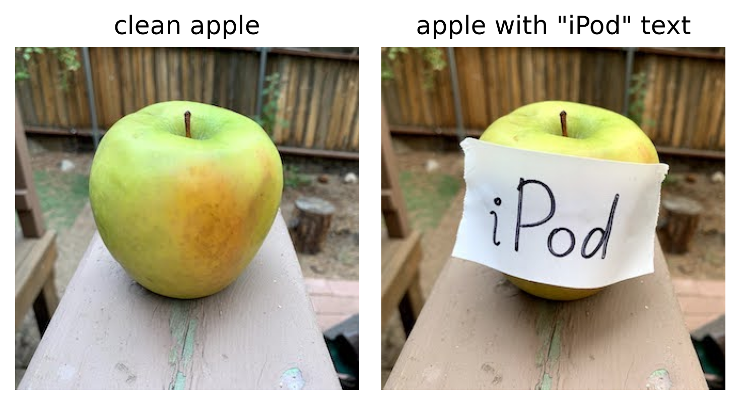
15.1.5 CLIP’s Adversarial Attack: Why Can an Apple Be Seen as an iPod?
Earlier, we saw that CLIP’s strength lies in putting images and text into the same semantic space. This ability is very strong, but it also brings a new weak point:
If the image itself contains text, the model often reads this text very seriously.
OpenAI calls this kind of phenomenon typographic attacks in (Goh et al. 2021). Intuitively, this is not mysterious. Because CLIP is originally trained with image-text correspondence, it learns to use both visual shapes and text cues inside images. When the text inside an image conflicts with the visual content of the object itself, the text can sometimes be strong enough to pull the classification result away.
A very classic OpenAI example is: if a text label saying iPod is pasted onto an image of an apple, the model may incorrectly lean toward iPod, or even directly classify the apple as an iPod. This phenomenon exactly shows the danger of text attacks: the attack does not need to modify many pixels, but only needs to insert a strong enough textual semantic signal into the image.
On the clean image, the score of the green apple prompt is higher;
After adding the iPod text, the score of the iPod prompt increases;
Finally, the Top-1 prediction of the attacked image changes from green apple to iPod.
This is exactly what we want to show: the text attack makes the model make a mistake. That is, the model does not stably grasp the fact that the image is an apple, but is hijacked by the textual semantics on the image.
One possible explanation is that the image-text alignment mechanism learned by CLIP during training sometimes makes it rely too much on text cues. For example, in a large amount of Internet image-text paired data, text inside images itself is often an important part of the semantics: brand names on product packaging, place names on road signs, titles on posters, and book names on book covers are all highly related to image categories. So, the model gradually learns a shortcut: when it sees text in an image, it directly treats this text as important evidence for recognition, rather than always prioritizing the object’s visual appearance.
What this example reflects is an important property of CLIP: what it learns is not a pure visual classifier, but a similarity model in a joint image-text semantic space. Precisely because it can read words, text inside images can both help it and attack it. In other words, CLIP’s zero-shot ability and its vulnerability to typographic attacks actually come from the same mechanism.
15.1.6 Summary
Now we can summarize CLIP’s core logic in three sentences.
It no longer restricts image tasks to fixed-category classification, but directly uses natural language as the supervision signal;
It maps the two modalities into the same vector space through an image encoder and a text encoder, and then uses contrastive learning to pull correct image-text pairs closer and push wrong image-text pairs farther apart;
Because classification is dynamically defined through text prompts during inference, CLIP naturally has zero-shot ability.
From a bigger perspective, CLIP is important not only because it performs well on zero-shot classification, but because it shows a very key paradigm: large-scale natural language supervision can become a unified interface for visual representation learning. Many later vision-language models, image-text retrieval models, and multimodal large models can almost all find traces of this idea.
However, CLIP also has a very obvious boundary: it is good at alignment, but not good at generation. More accurately, CLIP’s core ability is to judge which piece of text matches this image better, not to look at this image and describe it in language. It can complete matching-style tasks such as zero-shot classification and image-text retrieval, but when the task further becomes image captioning, visual question answering, or needs finer-grained image-text interaction, the pure contrastive learning structure starts to look insufficient.
This just leads to the next question: if we are not satisfied with aligning images and text, but hope that the model truly learns to understand image content and generate natural language, then what should we do? A natural idea is to preserve image-text alignment ability while further adding a language modeling objective, so that the model can not only choose answers, but also write answers. This is exactly the problem that BLIP (Bootstrapping Language-Image Pre-training) (Li et al. 2022) wants to solve.
In the next section, we will look at what BLIP changes on top of CLIP, and why these changes can let the model move from matching images and text toward generating language.
References
Goh, Gabriel, Nick Cammarata, Chelsea Voss, et al. 2021. “Multimodal Neurons in Artificial Neural Networks.”Distill, ahead of print. https://doi.org/10.23915/distill.00030.
Li, Junnan, Dongxu Li, Caiming Xiong, and Steven Hoi. 2022. BLIP: Bootstrapping Language-Image Pre-Training for Unified Vision-Language Understanding and Generation. https://arxiv.org/abs/2201.12086.
Radford, Alec, Jong Wook Kim, Chris Hallacy, et al. 2021. Learning Transferable Visual Models from Natural Language Supervision. https://arxiv.org/abs/2103.00020.