14.2 The Forward Process of DDPM: From Image to Noise
Author
jshn9515
Published
2026-03-31
Modified
2026-04-16
In the previous section, we first understood the core idea of DDPM from an intuitive perspective: first turn a real image into noise step by step, and then learn the reverse process of this process. If you have already accepted this general direction, then the next questions are:
How exactly is this noising process defined?
Why does it eventually become Gaussian noise?
Why does DDPM specifically design such a forward process?
In this section, we will make the forward diffusion process clear. This part is very important, because it almost determines the entire modeling framework of DDPM.
import randomimport timeimport dnnlpyimport matplotlib.pyplot as pltimport torchimport torchvision.datasets as datasetsimport torchvision.transforms.v2 as v2from torch import Tensorplt.rc('figure', dpi=100)print('PyTorch version:', torch.__version__)
PyTorch version: 2.12.1+cpu
14.2.1 The Process from Image to Noise: A Gaussian Markov Chain
Suppose we have a real image \(x_0\). We want to add noise step by step through several steps. Therefore, we can define a chained forward process:
Here, \(x_0\) is the real sample, \(x_t\) is the result after adding noise at step \(t\), and \(x_T\) is close to a standard Gaussian distribution.
So, through many small random perturbations, we gradually wash out the real data. In this way, the change at each step is very small, and the whole process is smoother and easier to analyze.
In DDPM, the forward process is usually written as a Markov chain:
When you first see this formula, it may feel a bit abstract. It is actually saying that the transition probability from \(x_{t-1}\) to \(x_t\) is not a deterministic function, but a Gaussian distribution. Its mean is \(\sqrt{1-\beta_t}\,x_{t-1}\), and its variance is \(\beta_t I\). In other words, \(x_t\) is obtained by adding Gaussian noise on top of \(x_{t-1}\).
Writing the formula above in a more familiar form, we get:
Here, \(\epsilon_t\) is a standard Gaussian noise; \(\beta_t \in (0,1)\) is the noising strength of this step; \(\sqrt{1-\beta_t}\) controls how much of the original image is retained; and \(\sqrt{\beta_t}\) controls how much noise is injected. In general, we control the range of \(\beta_t\) between 0.0001 and 0.02, and gradually increase it as \(t\) increases. This can ensure that the final \(x_T\) is close to a standard Gaussian distribution. Also, because \(\beta_t\) is very small, \(\sqrt{1-\beta_t}\) is close to 1, so at each step we keep most of the original image information and only mix in a little bit of noise.
So the essence of this formula is just one sentence: new image = keep most of the old image + mix in a small amount of random noise. This also matches the intuition from the previous section.
14.2.2 Why Multiply by \(\sqrt{1-\beta_t}\) in Front?
When many people first see this part, they will ask a natural question:
Why not simply write \(x_t = x_{t-1} + \text{noise}\)?
This is a very good question. In fact, if we simply stack noise on top at each step, the overall variance of the image will become more and more uncontrolled, and the numerical scale may keep expanding. Although the image can also become dirty this way, the process is not very stable and is not convenient to analyze. So DDPM uses a more regular design:
In this way, we can understand each step as a kind of controlled interpolation. From the perspective of variance, this form is also cleaner. Because if both \(x_{t-1}\) and \(\epsilon_t\) roughly have unit variance, then the variance of the first part is about \(1-\beta_t\), and the variance of the second part is about \(\beta_t\). Added together, they are still about 1.
So this design ensures that while noise is continuously added, the overall numerical scale will not go out of control. It also makes the training and inference processes of the network more stable and easier to analyze.
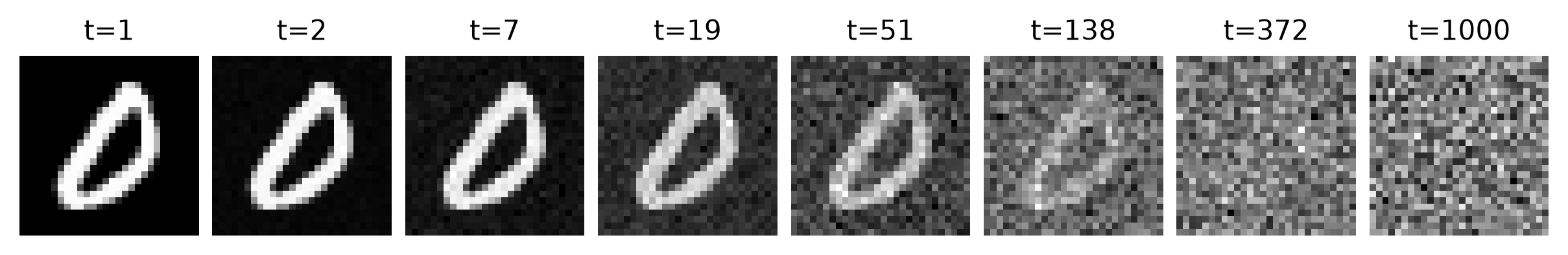
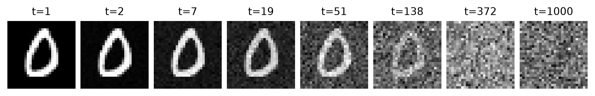
root = dnnlpy.get_data_root()transform = v2.Compose([v2.ToImage(), v2.ToDtype(torch.float32, scale=True)])ds = datasets.MNIST(root, train=False, download=True, transform=transform)idx = random.randrange(len(ds))x0 = ds[idx][0].squeeze(0) # shape: (28, 28)def add_noise_v1(x0: Tensor, betas: Tensor) -> Tensor: xt = x0.clone()for beta in betas: noise = torch.randn_like(x0) xt = (1- beta).sqrt() * xt + beta.sqrt() * noisereturn xtbetas = torch.linspace(0.0001, 0.02, steps=1000)samples = [x0]t1 = time.time()for i inrange(len(betas)): xt = add_noise_v1(x0, betas[:i +1]) samples.append(xt)t2 = time.time()print(f'[Time]: add_noise_v1 took {t2 - t1:.4f} seconds.')# We use step=8 here for better visualizationidx = torch.logspace(0, 3, steps=8, dtype=torch.long)samples = [samples[i] for i in idx -1]fig = plt.figure(1, figsize=(8, 2))axes = fig.subplots(1, len(samples))for i, ax inenumerate(axes): ax.imshow(samples[i], cmap='gray') ax.axis('off') ax.set_title(f't={idx[i]}', fontsize=10)fig.tight_layout(pad=0.5)dnnlpy.set_matplotlib_format('highdpi')plt.show()
[Time]: add_noise_v1 took 8.8308 seconds.
We perform 1000 such noising operations on the original image \(x_0\), and choose 8 different time points from steps 1 to 1000 to observe how the image changes. We will find that in the first few steps, the structure of the image is very clear; as the number of steps increases, the image gradually becomes blurry; after 300 steps, the original structure is already completely submerged in noise. The more noising steps there are, the closer the final image is to a Gaussian distribution, and the better the images obtained by reverse sampling will be.
This is exactly what the forward diffusion process wants to do.
14.2.3 The Role of \(\beta_t\) and Noise Scheduling Strategies
In the forward process, \(\beta_t\) represents the noise strength at step \(t\). It determines how aggressive this round of noising is.
If we set \(\beta_t\) for all steps to be very large, then the image will be destroyed very quickly, and the difference between two adjacent steps will be too drastic. This makes the reverse process harder to learn, because at each step the model has to correct a large amount of error. This is almost the same as directly generating an image from noise, and it loses the advantage of gradual correction. Conversely, if \(\beta_t\) at each step is relatively small, then the image is slowly pushed toward the noise distribution, and the whole process is smoother.
Therefore, DDPM usually sets a Noise Scheduler in advance:
\[
\beta_1, \beta_2, \dots, \beta_T
\]
This sequence of numbers is usually manually specified, not learned through training.
Common practices include:
Linear schedule: let \(\beta_t\) gradually increase over time. The example above uses this one;
Square-root linear schedule: let \(\sqrt{\beta_t}\) gradually increase over time;
Cosine schedule: let the overall noise injection process change in a cosine-like way.
The shared idea behind them is: add less noise in the early stage, and then gradually increase it later, so that the signal decays smoothly. Therefore, they are all monotonically increasing functions.
This formula is worth looking at several more times, because it is very important. For the full derivation of the formula, see (Luo 2022, eq. 61-70). Here, let us first understand this formula.
The first half of this formula, namely \(\sqrt{\bar{\alpha}_t}\,x_0\), represents how much of the original image \(x_0\) remains after \(t\) steps. Since \(\bar{\alpha}_t\) is the cumulative product of \(\alpha_t\), and \(\alpha_t = 1 - \beta_t\) is a number smaller than 1, \(\bar{\alpha}_t\) will gradually become smaller as \(t\) increases. This means that as time goes on, the weight of the original image becomes weaker and weaker.
This corresponds exactly to the effect we want: the later the time step, the less original structure remains in the image, and the more noise there is.
This shows that during training, we actually do not need to really simulate from \(x_0\) to \(x_t\) step by step. As long as we know the \(\bar{\alpha}_t\) corresponding to step \(t\), we can send the sample to any noise level in one shot. This makes training much more efficient.
14.2.5 Why Does It Eventually Approach Gaussian Noise?
This is a particularly key step when understanding DDPM.
As \(t\) keeps increasing, \(\bar{\alpha}_t\) will keep getting smaller. If we set the number of steps large enough and design the schedule properly, then in the end we will have:
In other words, at the final step, the original image information has almost completely disappeared, and only a variable approximately following standard Gaussian noise remains. In fact, it can be proved that when \(T \to \infty\), the distribution of \(x_T\) weakly converges to a standard Gaussian distribution. This is an asymptotic process, so in practice we only need \(T\) to be large enough to make \(x_T\) very close to a Gaussian distribution. Generally speaking, for DDPM, the value of \(T\) is usually around 1000.
So this is exactly the result DDPM wants most: gradually turn a complex data distribution into a very simple distribution that is very easy to sample from. As for why it becomes a Gaussian distribution: because the Gaussian distribution is a very simple distribution. We know its analytic form, can easily sample from it, and it is also mathematically easy to handle.
14.2.6 The Design Motivation of the DDPM Forward Process
At this point, you may notice that the forward process of DDPM is not designed casually. The reason it is often written as:
It is simple enough. Each step is a Gaussian perturbation, with a regular form, easy to implement and easy to derive.
It is smooth enough. Each step only adds a little bit of noise, so the change between adjacent states is not too drastic.
It has a closed-form expression. This is especially important. Because we can write \(x_t\) directly as a combination of \(x_0\) and noise, training becomes very convenient.
It turns the endpoint into a Gaussian distribution, and the Gaussian distribution is the easiest starting point for us to sample from. During generation, we only need to start from Gaussian noise and then learn to walk backward.
So we can say:
The forward process of DDPM is essentially a manually designed destruction process that is mathematically comfortable.
After saying so much, how exactly is this forward process used during training?
You may feel surprised when hearing it: the model actually does not need to learn the forward process at all. The definition of the forward process is fixed. Its only role is to create versions of training samples at different noise levels. During training, we can directly use the closed-form formula above to generate noisy images at different levels.
During training, we usually do the following:
Take a real image \(x_0\) from the dataset;
Randomly sample a time step \(t\);
Sample a standard Gaussian noise \(\epsilon\);
Use the formula \(x_t = \sqrt{\bar{\alpha}_t}x_0 + \sqrt{1-\bar{\alpha}_t}\epsilon\) to construct the corresponding noisy image;
Feed \(x_t\) and \(t\) to the neural network, and let it predict the noise \(\epsilon\).
So, the forward process plays the role of the problem setter in training. It is responsible for making the original image dirty, and it knows exactly how much noise was added. Then it asks the neural network to guess it back. Therefore, the training problem becomes a supervised learning problem: given an image at some noise level, can you predict the noise mixed into it?
This is much more concrete than directly asking the model to generate an image out of nothing.
14.2.7 Summary
At this point, we can compress the core content of 14.2 into a few sentences.
The forward process of DDPM is a Markov chain that gradually adds noise:
This allows training to randomly jump to any noise level, without really simulating step by step.
Then what about the reverse process? If the forward process adds noise, then the reverse process naturally removes noise. But why is predicting noise equivalent to denoising? Why does the training objective of DDPM eventually become a simple MSE? After understanding forward diffusion, the next step is to see how we can walk from noise back to an image step by step. This is where DDPM truly begins generation.