And as the number of steps increases, the structure in the image will gradually be drowned out by noise, and finally \(x_T\) will approach a standard Gaussian distribution.
Then, since we can add noise to an image step by step until it becomes Gaussian noise, can we walk back step by step from Gaussian noise?
This is the core question of the Reverse Diffusion Process.
In this section, we will clarify three things:
What the reverse process actually wants to learn;
Why it can be modeled as step-by-step denoising;
Why DDPM usually writes the training objective as noise prediction in the end.
import randomimport dnnlpyimport dnnlpy.models.ddpm.utils as dutilsimport matplotlib.pyplot as pltimport torchimport torchvision.datasets as datasetsimport torchvision.transforms.v2 as v2from torch import Tensorplt.rc('figure', dpi=100)dnnlpy.set_matplotlib_format('highdpi')print('PyTorch version:', torch.__version__)
PyTorch version: 2.12.1+cpu
14.3.1 If the Forward Process Can Move Forward, Why Can’t the Reverse Process Move Backward?
When many people first see this, they naturally have a question: since forward noise addition is so simple, can’t we just reverse it directly? Unfortunately, things are not that simple. Because adding noise itself is a process that loses information.
For example, if you have a clear image of a cat and add a little noise to it, you can still roughly tell that it is a cat. But if I only give you a noisy image, you cannot uniquely determine which clear image it originally came from. So, if we understand the reverse process as an inverse function transformation, we will find that it does not satisfy single-valuedness at all. In other words, the reverse process is one-to-many. Behind one noisy image, there may be many possible clear images.
Therefore, the reverse process cannot simply be understood as a deterministic inverse. A more reasonable way to understand it is:
Given the current noisy image \(x_t\), the next cleaner image \(x_{t-1}\) should follow some conditional probability distribution.
We denote this conditional distribution as \(q(x_{t-1} \mid x_t)\). That is, given the noisy image \(x_t\) at the current step \(t\), the model needs to give the probability distribution of the cleaner sample \(x_{t-1}\) from the previous step. It describes the single-step reverse distribution corresponding to the real diffusion process. Then, there is a problem here: is this distribution easy to obtain?
The forward distribution \(q(x_t \mid x_{t-1})\) is designed by ourselves, so this part is easy. But what about \(q(x_{t-1})\) and \(q(x_t)\)? They correspond to the marginal distributions of samples at step \(t-1\) and step \(t\), respectively. That is:
You see, both of them involve the real data distribution \(q(x_0)\), and the real data distribution is something we cannot directly model. If we already knew it, why would we need DDPM? So this reverse conditional distribution \(q(x_{t-1} \mid x_t)\) is a very complex distribution, and we cannot directly compute it at all.
Then what should we do? Don’t forget that we have real images! Can we use them?
Of course. Although \(q(x_{t-1} \mid x_t)\) is complex, if we write the distribution in this form:
You will find that the three terms on the right are all known! The first two terms are the forward process designed by ourselves, and the last term \(q(x_t \mid x_0)\) can also be obtained through the recurrence relation of the forward process. In other words, although \(q(x_{t-1} \mid x_t)\) is complex, \(q(x_{t-1} \mid x_t, x_0)\) is a simple distribution. We can directly derive its analytic expression, and then step by step obtain the conditional distribution of the reverse process.
In fact, it can be proved that under the definition of the forward process, the reverse conditional distribution \(q(x_{t-1} \mid x_t, x_0)\) is a Gaussian distribution:
For the full proof, see (Luo 2022, eq. 71-84). Note that the result here is a little different from the result in the paper. The paper ignores some constant terms, so it writes “proportional to”; here we have written the constant terms as well.
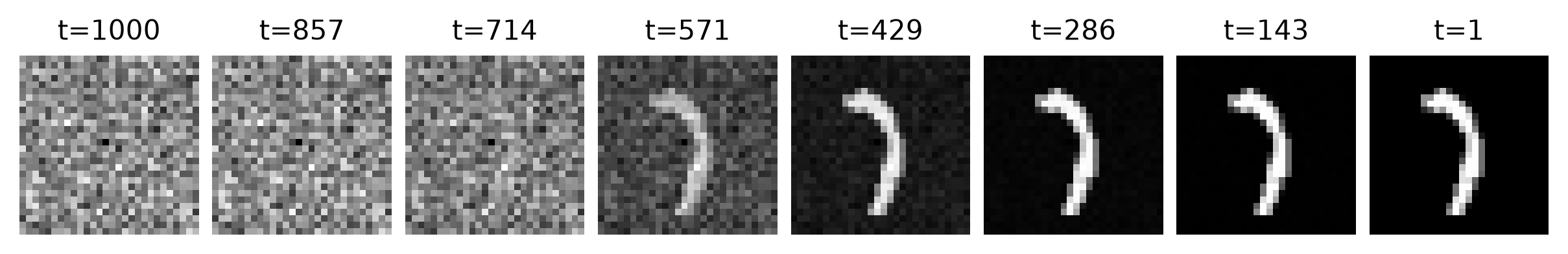
Now let’s do an experiment. Using the MNIST dataset, suppose we have the original image \(x_0\). We first add noise to one image according to the forward formula until it becomes Gaussian noise, and then walk back step by step from Gaussian noise. Let’s see how the image changes during this process.
root = dnnlpy.get_data_root()transform = v2.Compose([v2.ToImage(), v2.ToDtype(torch.float32, scale=True)])ds = datasets.MNIST(root, train=False, download=True, transform=transform)idx = random.randrange(len(ds))x0 = ds[idx][0].squeeze(0) # shape: (28, 28)def denoise_v1(x0: Tensor, xt: Tensor, timestep: int, betas: Tensor) -> Tensor: t = timestep alphas =1.0- betas alpha_t = alphas[t] alpha_bars = alphas.cumprod(dim=0) alpha_bar_t = alpha_bars[t] alpha_bar_prev_t = alpha_bars[t -1] if t >0else torch.tensor(1.0) beta_t = betas[t] param1 = alpha_bar_prev_t.sqrt() * beta_t / (1- alpha_bar_t) param2 = alpha_t.sqrt() * (1- alpha_bar_prev_t) / (1- alpha_bar_t) mean = param1 * x0 + param2 * xt variance = (1- alpha_bar_prev_t) / (1- alpha_bar_t) * beta_tif t >0:return mean + variance.sqrt()else:return meanT =1000betas = torch.linspace(0.0001, 0.02, steps=T)xt = dutils.add_noise(x0, betas, T -1)trajectory = [xt.clone()]for t inrange(T -1, -1, -1): xt = denoise_v1(x0, xt, t, betas) trajectory.append(xt.clone())# We use step=8 here for better visualizationidx = torch.linspace(1000, 1, steps=8, dtype=torch.long)trajectory = [trajectory[T - i] for i in idx -1]fig = plt.figure(1, figsize=(8, 2))axes = fig.subplots(1, len(trajectory))for i, ax inenumerate(axes): ax.imshow(trajectory[i], cmap='gray') ax.axis('off') ax.set_title(f't={idx[i]}', fontsize=10)fig.tight_layout(pad=0.5)plt.show()
You see, we successfully recovered the original image! However, there is another problem here: during the process of recovering the image, we used the original image \(x_0\). But generating images is exactly about generating \(x_0\). If we already know \(x_0\), then what are we still generating?
This is where neural networks come in. We define a parameterized conditional distribution \(p_\theta(x_{t-1} \mid x_t)\) and let it approximate \(q(x_{t-1} \mid x_t, x_0)\).
In essence, what the reverse process needs to learn is the reverse conditional distribution at each step:
\[
p_\theta(x_{t-1} \mid x_t)
\]
That is, given the noisy image \(x_t\) at the current step \(t\), the model needs to give the probability distribution of the cleaner sample \(x_{t-1}\) from the previous step.
Then the whole generation chain can be written as:
The starting point \(p(x_T)\) is very simple. Usually, we directly take the standard Gaussian distribution \(\mathcal{N}(0, I)\). The difficulty is all concentrated on the reverse conditional distribution \(p_\theta(x_{t-1} \mid x_t)\) at each step. So, what does this distribution look like? And how should we learn it?
In the previous section, we knew that the reverse conditional distribution \(q(x_{t-1} \mid x_t, x_0)\) is essentially a Gaussian distribution:
That is, if we directly fix the covariance as \(\tilde{\beta}_t I\), it is already enough. So in actual training, we usually only let the model predict the mean \(\mu_\theta(x_t, t)\), and fix the covariance \(\Sigma_\theta(x_t, t)\) as \(\tilde{\beta}_t I\).
14.3.3 Why Is It Finally Often Written as Noise Prediction?
At this point, you may feel that since the reverse distribution is Gaussian and the model mainly learns the mean \(\mu_\theta(x_t, t)\), can’t we just directly predict this mean during training?
In theory, of course we can. But in practice, DDPM usually adopts a more clever and more stable parameterization:
It does not directly predict the mean, but predicts the noise \(\epsilon\) mixed into the current sample.
That is, we let the model learn:
\[
\epsilon_\theta(x_t, t)
\]
The reason is also simple. We know that the expression of the true mean \(\tilde{\mu}_t(x_t, x_0)\) actually contains the original image \(x_0\):
So, if we want to predict this mean accurately, since the mean itself depends on \(x_0\), the model is actually indirectly recovering information about the original image. Instead of directly predicting such a complex mean whose form changes with the timestep, we would rather rewrite the learning target into a simpler and more stable form.
We know that the forward process has a closed-form sampling formula:
That is, the current noisy image \(x_t\) is formed by mixing the original image \(x_0\) and noise \(\epsilon\). We can transform this equation a little:
The noise \(\epsilon\) here is sampled by ourselves during training, so it is known. In this way, we can use the noise as the model’s training target, let the model predict it, indirectly obtain an estimate of the original image \(x_0\), and finally obtain the mean \(\mu_\theta(x_t, t)\). At the same time, we also avoid the trouble of directly predicting a complex mean that changes with the timestep. Besides, predicting noise and predicting the mean are essentially equivalent.
So the final training objective of DDPM is usually written as:
The derivation here is not rigorous. We only explain intuitively why noise prediction is reasonable, and we have not strictly explained its theoretical basis. From the perspective of rigorous probabilistic modeling, the training objective of DDPM actually comes from the variational lower bound (ELBO), and the common noise prediction loss is an equivalent or approximately equivalent rewriting based on that objective. We will not expand the full derivation here for now, and will explain it in detail later. Interested readers can first look at (Luo 2022, eq. 46-58, 115-130).
14.3.4 DDPM’s Training Objective: A Very Simple MSE
In the previous section, we wrote the training objective of DDPM as a mean squared error for noise prediction:
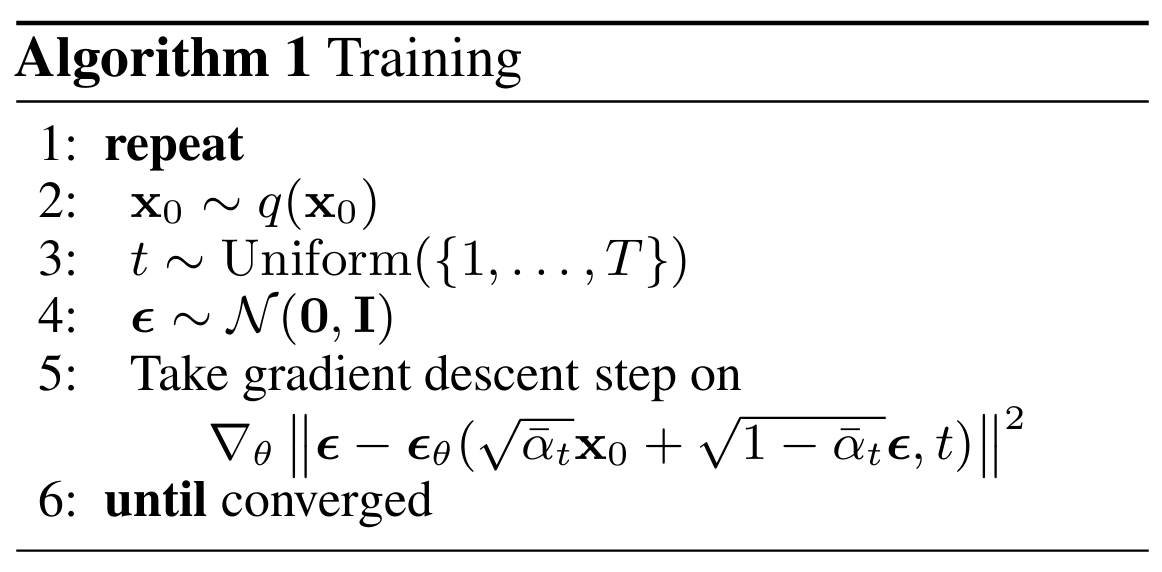
Here, \(x_0\) is sampled from the real data \(p_{\text{data}}\), \(t\) is a randomly selected timestep from 1 to \(T\), and \(\epsilon\) is Gaussian noise sampled by ourselves. This loss function looks a bit too simple: the whole diffusion model often ends up just doing a mean squared error for noise regression.
However, although it looks like just MSE on the surface, behind it is actually probabilistic modeling of the reverse diffusion process. In other words, this simple MSE loss function actually starts from a rigorous probabilistic model, goes through a series of equivalent or approximately equivalent transformations, and finally becomes a training objective that is very easy to optimize. Unlike many deep learning networks, it has theoretical support behind it. We use a piece of pseudocode to describe this process:
Algorithm 14.3.4: DDPM training process pseudocode (Ho et al. 2020, alg. 1)
You see, isn’t it simple? Don’t be fooled by it. Later, we will explain in detail where this training objective comes from and how it relates to probabilistic modeling.
14.3.5 Summary
At this point, we can connect Sections 14.1, 14.2, and 14.3 together.
Step 1: Define forward noise addition
We manually design a fixed process that turns real data into noise step by step:
Step 3: Model the reverse process as conditional Gaussian distributions
Each step is not a direct inverse, but learns:
\[
p_\theta(x_{t-1} \mid x_t)
\]
Step 4: Turn the training objective into noise prediction
Using the closed-form formula of the forward process, we can directly construct the supervision signal and let the model learn:
\[
\epsilon_\theta(x_t, t)
\]
This turns a complex generative modeling problem into a noise regression problem that can be optimized stably.
This logical chain is the most basic DDPM training framework.
At this point, we finally understand the training and sampling process of DDPM. However, there are still many details we have not clarified. For example, how should the timestep \(t\) in the model input be represented? Why is U-Net especially suitable as a denoising network? During sampling, how exactly do we compute \(x_{t-1}\) from \(x_t\)? These are what we will look at in the next section, where we discuss some detailed designs of DDPM.