In the previous sections, we have already built up the most core ideas of DDPM:
First define a forward noising process, turning a real image into noise step by step;
Then learn a reverse process, walking from noise back to data step by step;
During training, the model usually does not directly predict the original image, but predicts the noise in the current step.
However, we have not really implemented these ideas into a concrete network structure and sampling process yet. For example, we know the model needs to predict noise, but what is its input? What is its output? How is the timestep \(t\) told to the network? Why do many implementations like to use U-Net? How is sampling iterated?
In this section, we explain the overall running process of DDPM from the perspective of engineering implementation.
import mathimport randomimport dnnlpyimport dnnlpy.models.ddpm as ddpmimport matplotlib.pyplot as pltimport numpy as npimport torchimport torch.nn as nnimport torch.nn.functional as Fimport torch.utils.data as utilsimport torchvision.datasets as datasetsimport torchvision.transforms.v2 as v2from dnnlpy.models.ddpm import DDPMScheduler, UNet2DModelfrom torch import Tensorplt.rc('figure', dpi=100)print('PyTorch version:', torch.__version__)
14.4.1 Timestep \(t\): Letting the Network Know Which Step It Is Currently at
Let’s first recall the training task. We start from a real image \(x_0\), randomly sample a timestep \(t\), and then construct the noisy image \(x_t\) according to the forward process. Next, we input \((x_t, t)\) into the neural network and let it predict the noise in the current step:
\[
\epsilon_\theta(x_t, t)
\]
So, we need to input a noisy image \(x_t\) and the current timestep \(t\), and let the network output the noise estimate \(\epsilon_\theta(x_t, t)\) contained in this image. If this noise estimate is accurate enough, we can follow the reverse formula and push the image one step in a cleaner direction.
Then, suppose you only input \(x_t\) into the network without telling it which step it is currently at. What will happen?
The answer is that the network will be very confused. Because the noise intensity of images at different timesteps is very different. In early timesteps, the image is still relatively clear and only has a little noise; in middle timesteps, the image has already become very blurry, and structure and noise are mixed together; in later timesteps, the image is almost pure noise. In these three cases, how much noise should be removed and how much structure should be kept are completely different tasks. If we do not tell the network which step it is currently at, it has to guess the noise level only from the input image itself, which greatly increases the learning difficulty.
So in DDPM, the model is generally written as:
\[
\epsilon_\theta(x_t, t)
\]
That is to say, the timestep \(t\) is part of the model input. This is a kind of conditional information. It tells the network how strong the noise is now, and lets the network know how large a correction it should make at the current moment, so that the same network can handle denoising tasks under different noise levels.
So DDPM is actually a conditional denoiser, and the condition is the current timestep \(t\).
14.4.2 Timestep Embedding: Vector Representation of Time Information
Now that we have the timestep \(t\), the next question is: an image is a tensor, while the timestep \(t\) is only an integer. How do we turn this integer into information that the neural network can effectively use?
The simplest method is to normalize \(t\) into a scalar and concatenate it in. But in practice, this is usually not good enough. Because the relationship between different timesteps is not linear, the network needs a richer representation to distinguish different noise stages. Using only one number makes it difficult to express the complex differences between early, middle, and late stages. Because the network does not naturally understand that “100 is larger than 10”; it can only learn this relationship through training data, and this increases the learning difficulty.
So many diffusion models use a method very similar to positional encoding in Transformer, which maps the timestep \(t\) into a high-dimensional vector. This is usually called Time Embedding. The dimension of this vector can be the same as the dimension of the image features, so it can be directly concatenated with them and input into the network.
One common method is to use sinusoidal and cosine-form encoding:
Then it passes through several MLP layers and becomes a feature vector suitable for the current network width.
In this way, different timesteps will be mapped to different positions, and the representations of nearby timesteps also maintain a certain smoothness. The network can more easily learn what strategy it should take at different noise stages. This is a bit similar to positional encoding in Transformer. There, we tell the model the position of the current token in the sequence. In diffusion models, we tell the model the stage of the current image in the denoising chain.
Tip
About why positional encoding and timestep embedding both like to use sinusoidal and cosine functions, you can review the analysis of positional encoding in Section 8.4. Simply speaking, sinusoidal and cosine functions allow the representations of different timesteps to be distributed regularly in space, and also let the representations of nearby timesteps maintain a certain smoothness. This helps the network learn strategies for different noise stages.
Each row in this figure represents the encoding result of one timestep, and each column represents the value change of one encoding dimension across different timesteps. Some columns change color quickly, which means these dimensions correspond to higher frequencies and are more sensitive to small changes in the timestep; some columns change more slowly, which means these dimensions correspond to lower frequencies and can provide smoother, coarser-grained time information.
Therefore, encoding dimensions with different frequencies together form a multi-scale time representation. This allows the network to both perceive small differences between timesteps and grasp the overall noise stage it is currently in. With the help of this time encoding, the network can distinguish different timesteps and learn to adopt different denoising strategies under different noise levels.
14.4.3 U-Net: The Classic Choice for the Denoising Network
At this point, we already know what the input and output are. The next question is, what structure should the denoising network use?
In theory, many networks can be tried. But in image diffusion models, the most classic and most common choice is U-Net. This is because U-Net is very suitable for this kind of task where the input is an image and the output is an image of the same size (Ronneberger et al. 2015).
The input of DDPM is \(x_t\), and the output is usually a noise tensor \(\hat{\epsilon}\) with the same size as the image. That is to say, the model needs to give a prediction for every pixel position, and it also needs to understand both local texture information and global structure information. The design of U-Net exactly meets this need.
14.4.3.1 Review of the Basic Idea of U-Net
In semantic segmentation, we explained the structure of U-Net in detail. Here we briefly review its core idea.
The name U-Net comes from its shape. It is generally divided into two parts:
Downsampling path (encoder): continuously compresses the resolution and extracts higher-level features with larger receptive fields;
Upsampling path (decoder): gradually restores the spatial resolution and turns abstract features back into pixel-level output.
In the middle, skip connections are added to directly pass early high-resolution features to the later upsampling layers.
Doing this has several obvious benefits:
The downsampling stage can see a larger range of context and understand the overall structure;
The upsampling stage can recover spatial details;
Skip connections can preserve shallow local texture and edge information.
And denoising itself requires looking at both the global and local levels. Globally, we need to know roughly what structure this image has; locally, we need to know how the noise near a certain pixel should be corrected. So U-Net and the task of diffusion models naturally fit very well.
14.4.3.2 How Is Timestep Information Integrated into U-Net?
Earlier, we said that besides the image \(x_t\), the model must also know the current timestep \(t\). Then in U-Net, how is this time information usually integrated?
A common method is:
First turn \(t\) into a time embedding vector;
Then use a small MLP to transform it into a suitable dimension;
Add this vector to the features of each layer, or use it to modulate the activations of each layer.
Of course, in more modern diffusion models, besides time embedding, category conditions and text conditions are also often added, or external information is integrated into the network through cross-attention. But in the most basic DDPM scenario, time embedding + U-Net is already a very classic combination.
UNet2DModel: a U-Net structure for 2D image denoising
class UNet2DModel(nn.Module):def__init__(self, in_channels: int=3, out_channels: int=3, block_out_channels: tuple[int, ...] = (64, 128, 256, 512), time_emb_dim: int=256, ):super().__init__()self.time_embedding = nn.Sequential( SinusoidalTimestepEmbedding(time_emb_dim), nn.Linear(time_emb_dim, time_emb_dim), nn.SiLU(), nn.Linear(time_emb_dim, time_emb_dim), ) first_ch = block_out_channels[0]self.init_conv = nn.Conv2d( in_channels, first_ch, kernel_size=3, padding=1, )# Down pathself.downs = nn.ModuleList() in_ch = block_out_channels[0] skip_channels = []for out_ch in block_out_channels: is_last_ch = out_ch == block_out_channels[-1]self.downs.append( nn.ModuleList( [ ResBlock(in_ch, out_ch, time_emb_dim), ResBlock(out_ch, out_ch, time_emb_dim), AttentionBlock(out_ch), Downsample(out_ch) ifnot is_last_ch else nn.Identity(), ] ) ) in_ch = out_ch skip_channels.append(out_ch)# Middle last_ch = block_out_channels[-1]self.mid_block1 = ResBlock(last_ch, last_ch, time_emb_dim)self.mid_attn = AttentionBlock(last_ch)self.mid_block2 = ResBlock(last_ch, last_ch, time_emb_dim)# Up pathself.ups = nn.ModuleList() in_ch = block_out_channels[-1]for out_ch inreversed(skip_channels): is_first_ch = out_ch == skip_channels[0]self.ups.append( nn.ModuleList( [ ResBlock(in_ch + out_ch, out_ch, time_emb_dim), ResBlock(out_ch, out_ch, time_emb_dim), AttentionBlock(out_ch), Upsample(out_ch) ifnot is_first_ch else nn.Identity(), ] ) ) in_ch = out_chself.final_block = ConvBlock(in_ch, in_ch)self.final_conv = nn.Conv2d(in_ch, out_channels, kernel_size=1)def forward(self, x: Tensor, timesteps: Tensor) -> Tensor:if x.size(0) != timesteps.size(0):raiseAssertionError(f'Batch size of x and timesteps must match, 'f'but got {x.size(0)} and {timesteps.size(0)}.' ) t_emb =self.time_embedding(timesteps) x =self.init_conv(x) skips = []for block1, block2, attn, down inself.downs: # type: ignore x = block1(x, t_emb) x = block2(x, t_emb) x = attn(x) skips.append(x) x = down(x) x =self.mid_block1(x, t_emb) x =self.mid_attn(x) x =self.mid_block2(x, t_emb)for block1, block2, attn, up inself.ups: # type: ignore skip = skips.pop() x = torch.concat([x, skip], dim=1) x = block1(x, t_emb) x = block2(x, t_emb) x = attn(x) x = up(x) x =self.final_block(x) x =self.final_conv(x)return x
14.4.4 DDPM Sampling Process: Step-by-Step Denoising + a Little Randomness at Each Step
After training is finished, the model has learned to predict noise under different timesteps. So during generation, we can do this:
First start from pure Gaussian noise \(x_T \sim \mathcal{N}(0, I)\);
Input \((x_T, T)\), and the model predicts the noise;
Based on this noise estimate, construct \(x_{T-1}\);
Then input \((x_{T-1}, T-1)\) and continue denoising;
Repeat until we obtain \(x_0\).
So generation is not completed in one step, but is a step-by-step denoising process. This also explains two typical characteristics of diffusion models:
High generation quality: because each step only makes a small correction;
Slow sampling speed: because it really needs to go through many, many steps.
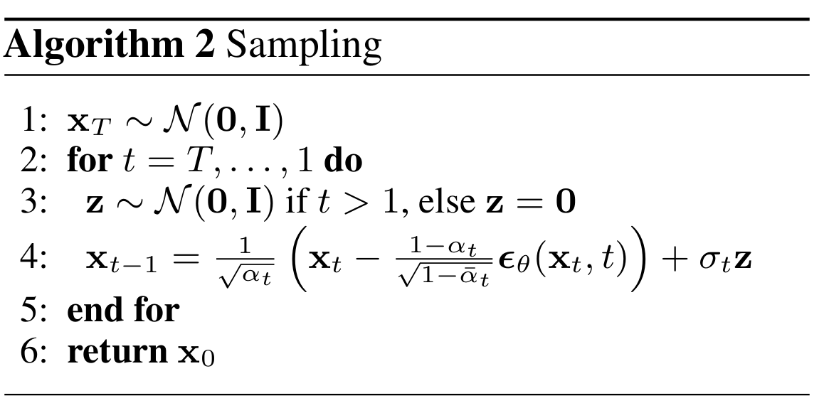
This is the pseudocode for the generation stage, and it is also very simple:
Algorithm 14.4.4: DDPM generation process pseudocode (Ho et al. 2020, alg. 2)
If you look carefully at this pseudocode, you will find that we seem to also add noise during the sampling process, which is the \(z\) in the pseudocode. But aren’t we already trying to generate an image? Why do we still add noise while denoising at each step?
We know that the reverse process is generally written as a Gaussian distribution:
This is a probability distribution. This means that the process from \(x_t\) to \(x_{t-1}\) not only has a mean, but also has a certain amount of randomness. So, in order to reflect this randomness, during sampling we often move along the mean direction given by the model while adding a little random perturbation. In other words, the sampling process at each step is:
If there is no randomness at all, the sampling path may become too rigid. Properly keeping some random perturbation is more consistent with the definition of the original probabilistic model. That is to say, the sampling process of DDPM is essentially also a stochastic process, not a completely deterministic process.
Of course, later there were also many variants, such as DDIM, that rewrote the random sampling process of DDPM into an update process that can be deterministic. But in the most basic DDPM, step-by-step sampling + a little randomness at each step is the standard practice.
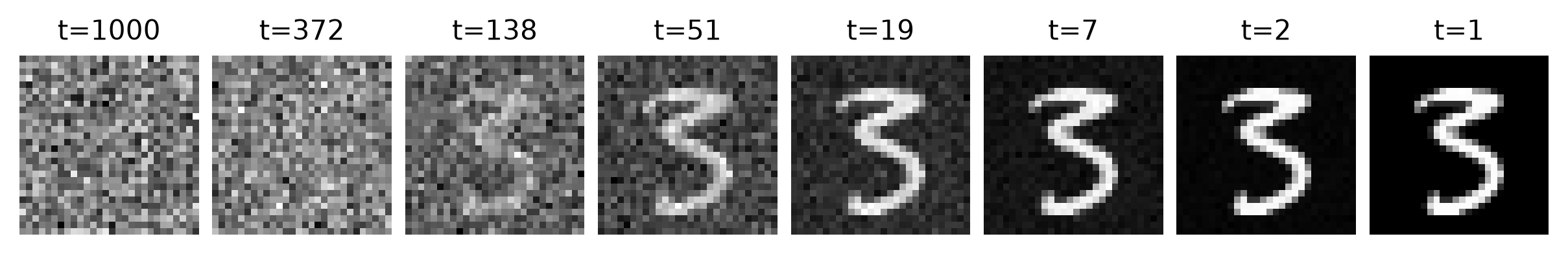
root = dnnlpy.get_data_root()transform = v2.Compose([v2.ToImage(), v2.ToDtype(torch.float32, scale=True)])ds = datasets.MNIST(root, train=False, download=True, transform=transform)idx = random.randrange(len(ds))x0 = ds[idx][0].squeeze(0) # shape: (28, 28)def denoise_v2(x0: Tensor, xt: Tensor, timestep: int, betas: Tensor) -> Tensor: t = timestep alphas =1.0- betas alpha_t = alphas[t] alpha_bars = alphas.cumprod(dim=0) alpha_bar_t = alpha_bars[t] alpha_bar_prev_t = alpha_bars[t -1] if t >0else torch.tensor(1.0) beta_t = betas[t] param1 = alpha_bar_prev_t.sqrt() * beta_t / (1- alpha_bar_t) param2 = alpha_t.sqrt() * (1- alpha_bar_prev_t) / (1- alpha_bar_t) mean = param1 * x0 + param2 * xt variance = (1- alpha_bar_prev_t) / (1- alpha_bar_t) * beta_tif t >0:# Add noise for all steps except the last one z = torch.randn_like(x0)return mean + variance.sqrt() * zelse:return meanT =1000betas = torch.linspace(0.0001, 0.02, steps=T)xt = ddpm.add_noise(x0, betas, T -1)trajectory = [xt.clone()]for t inrange(T -1, -1, -1): xt = denoise_v2(x0, xt, t, betas) trajectory.append(xt.clone())# We use step=8 here for better visualizationidx = torch.logspace(3, 0, steps=8, dtype=torch.long)trajectory = [trajectory[T - i] for i in idx -1]fig = plt.figure(2, figsize=(8, 2))axes = fig.subplots(1, len(trajectory))for i, ax inenumerate(axes): ax.imshow(trajectory[i], cmap='gray') ax.axis('off') ax.set_title(f't={idx[i]}', fontsize=10)fig.tight_layout(pad=0.5)dnnlpy.set_matplotlib_format('highdpi')plt.show()
14.4.5 Simplified Code for DDPM Training and Sampling
At this point, we can write out the entire DDPM implementation process using PyTorch code. To make it convenient to introduce the Hugging Face diffusers library later, the API here stays consistent with the design of diffusers.
14.4.5.1 Training Process
The training process is mainly divided into the following steps:
Sample a real image \(x_0\) from the dataset;
Randomly sample a timestep \(t\);
Sample a noise \(\epsilon\) from a Gaussian distribution;
According to the forward process formula, construct the noisy image \(x_t\);
Input \(x_t\) and \(t\) into the model to obtain the noise prediction \(\hat{\epsilon}\);
Compute the loss and update the model parameters.
The add_noise() function here is the add_noise_v2() function we defined in the previous sections. It uses the closed-form formula of the forward process to combine \(x_0\) and \(\epsilon\), and directly constructs \(x_t\) according to any timestep \(t\). The add_noise() function also additionally adds support for the batch dimension, so that batch data can be processed in actual training and training efficiency can be improved.
data = torch.randn(32, 3, 32, 32)train_ds = utils.TensorDataset(data)train_dl = utils.DataLoader(train_ds, batch_size=16, shuffle=True)model = UNet2DModel().to(device)scheduler = DDPMScheduler()model.train()# 1. Iterate over the training data.for x0, *_ in train_dl: x0 = x0.to(device) # [B, C, H, W]# 2. Sample random time steps for each image in the batch. timesteps = torch.randint( scheduler.num_train_timesteps, (x0.size(0),), dtype=torch.long, device=device, )# 3. Sample noise to add to the images. noise = torch.randn_like(x0)# 4. Add noise to the clean images according to the sampled time steps. xt = scheduler.add_noise(x0, noise, timesteps)# 5. Predict the noise using the model. pred_noise = model(xt, timesteps)# 6. Compute the loss between the predicted noise and the actual noise. loss = F.mse_loss(pred_noise, noise) loss.backward()print('Training step completed, loss:', loss.item())
Training step completed, loss: 1.0202131271362305
14.4.5.2 Sampling Process
The sampling process is mainly divided into the following steps:
Sample a noise image \(x_T\) from the standard normal distribution;
Set the timestep sequence, for example \(T, T-1, \dots, 1\);
For each timestep \(t\), construct a batch vector \(t_{batch}\) whose elements are all \(t\);
For the current \(x_t\) and \(t_{batch}\), input them into the model to obtain the noise prediction \(\hat{\epsilon}\);
According to the reverse process formula, compute \(x_{t-1}\), and maybe add random perturbation;
Finally obtain \(x_0\), which is the generated image.
The step() function here is the denoise_v2() function we defined in the previous sections. It computes the mean and variance of \(x_{t-1}\) according to the reverse process formula, and decides whether to add random perturbation according to whether the current denoising step is the last step. The step() function also additionally adds support for the batch dimension, so that batch data can be processed during actual sampling and sampling efficiency can be improved.
# 1. Start from pure noise (e.g., a random tensor).xt = torch.randn(1, 3, 32, 32, device=device)# 2. Set the number of inference timesteps.# Usually less than the number of training timesteps, e.g., 100.scheduler.set_timesteps(100, device=device)model.eval()with torch.inference_mode():for t in scheduler.timesteps:# 3. Construct a batch of time steps (same time step for the whole batch). t_batch = torch.full((xt.size(0),), int(t), dtype=torch.long, device=device)# 4. Predict the noise using the model. pred_noise = model(xt, t_batch)# 5. Compute the previous sample using the scheduler's step function. xt = scheduler.step(pred_noise, int(t), xt)# 6. The final sample after the last time step is the generated image.print(xt.shape)
torch.Size([1, 3, 32, 32])
Actually, from the sampling process, it is not difficult to see why DDPM sampling is usually relatively slow. Because it is not generated in one step, but needs to run many steps, and each step requires one U-Net forward pass, so the overall generation cost is relatively high. However, it is exactly because of this gradual process that DDPM can generate images with very high quality.
14.4.6 Summary
In this section, we looked at the network structure and sampling process of DDPM from the implementation perspective. It can be summarized in the following few sentences:
The network of DDPM does not directly generate images, but predicts noise at each step;
The model must know the current timestep, so time embedding is a key component;
U-Net is very suitable for this pixel-level, conditional, multi-scale denoising task;
During sampling, it starts from pure noise, repeatedly calls the same denoising network, and obtains the final image step by step.
At this point, how DDPM is done is basically complete. However, so far, we have not really understood it from the perspective of probabilistic modeling. Is the training objective of DDPM just an engineering trick? Or can it actually be derived from a strict probabilistic model objective?
In the next section, we will return to the perspective of probabilistic modeling and see how the objective function of DDPM is derived step by step from ELBO, and why it finally simplifies into the noise prediction loss we see now.
Ronneberger, Olaf, Philipp Fischer, and Thomas Brox. 2015. U-Net: Convolutional Networks for Biomedical Image Segmentation. https://arxiv.org/abs/1505.04597.