前面几节里,我们已经把 DDPM 最核心的想法搭起来了:
先定义一个前向加噪过程,把真实图像一步一步变成噪声;
再学习一个反向过程,从噪声一步一步走回数据;
训练时,模型通常不是直接预测原图,而是去预测当前这一步中的噪声。
但是,我们还没有真正把这些想法落实到一个具体的网络结构和采样流程中来。比如,我们知道模型要预测噪声,但它的输入是什么?它的输出是什么?时间步 \(t\) 怎么告诉网络?为什么很多实现喜欢用 U-Net?采样时又是怎么迭代的?
这一节,我们从工程实现的角度,把 DDPM 的整体运行方式讲清楚。
import mathimport randomimport dnnlpyimport dnnlpy.models.ddpm as ddpmimport matplotlib.pyplot as pltimport numpy as npimport torchimport torch.nn as nnimport torch.nn.functional as Fimport torch.utils.data as utilsimport torchvision.datasets as datasetsimport torchvision.transforms.v2 as v2from dnnlpy.models.ddpm import DDPMScheduler, UNet2DModelfrom torch import Tensor'figure' , dpi= 100 )print ('PyTorch version:' , torch.__version__)
PyTorch version: 2.12.1+cpu
= dnnlpy.get_default_device()print ('Using device:' , device)
14.4.1 时间步 \(t\) :让网络知道现在是第几步
我们先回忆一下训练时的任务。我们会从真实图像 \(x_0\) 出发,随机采样一个时间步 \(t\) ,然后按照前向过程构造出带噪图像 \(x_t\) 。接着,把 \((x_t, t)\) 输入神经网络,让它预测当前这一步里的噪声:
\[
\epsilon_\theta(x_t, t)
\]
所以,我们需要输入一张带噪图像 \(x_t\) 和当前时间步 \(t\) ,让网络输出这张图像中包含的噪声估计 \(\epsilon_\theta(x_t, t)\) 。如果这个噪声估计足够准确,我们就能按照反向公式,把图像往更干净的方向推一步。
那么,假设你只把 \(x_t\) 输入给网络,而不告诉它当前是第几步,会发生什么?
答案是,网络会很困惑。因为不同时间步的图像噪声强度差别非常大。在早期时间步,图像还比较清晰,只是稍微有一点噪声;在中间时间步,图像已经很模糊,结构和噪声混在一起;在后期时间步,图像几乎就是纯噪声。这三种情况下,该去掉多少噪声,该保留多少结构是完全不同的任务。如果不告诉网络当前是第几步,它就必须仅靠输入图像本身去猜测噪声级别,这会大大增加学习难度。
所以在 DDPM 里,模型一般都写成:
\[
\epsilon_\theta(x_t, t)
\]
也就是说,时间步 \(t\) 是模型输入的一部分。这是一种条件信息。它告诉网络现在噪声有多强,让网络知道当前应该做多大幅度的修正,从而让同一个网络可以处理不同噪声水平下的去噪任务。
所以 DDPM 实际上是就是一个条件去噪器(conditional denoiser),条件就是当前的时间步 \(t\) 。
14.4.2 时间步嵌入:时间信息的向量表示
有了时间步 \(t\) ,那接下来的问题就是:图像是一个张量,时间步 \(t\) 只是一个整数。怎么把这个整数变成神经网络能有效利用的信息?
最简单的方法就是把 \(t\) 归一化成一个标量,然后拼进去。但实践里,这样通常不够好。因为不同时间步之间的关系不是线性的,网络需要一种更丰富的表示,来区分不同的噪声阶段。仅用一个数字,很难表达早期、中期、后期的复杂差别。因为网络不会天然理解“100 比 10 更大”,它只能通过训练数据去学习这个关系,而这会增加学习难度。
所以很多扩散模型都会使用一种和 Transformer 里位置编码很像的方法,就是把时间步 \(t\) 映射成一个高维向量,这通常叫做 时间步嵌入(Time Embedding) 。这个向量的维度可以和图像特征的维度一样,这样就可以直接拼接在一起输入网络。
一种常见做法是使用正弦余弦形式的编码:
\[
\text{emb}(t) = [\sin(\omega_1 t), \cos(\omega_1 t), \sin(\omega_2 t), \cos(\omega_2 t), \dots]
\]
然后再经过几层 MLP,把它变成适合当前网络宽度的特征向量。
这样,不用同时间步就会被映射到不同的位置,相近时间步的表示也保持一定平滑性。网络更容易学到不同噪声阶段应该采取什么策略。这和 Transformer 里的位置编码有一点像。在那里,我们告诉模型当前 token 在序列中的位置。而在扩散模型里,我们告诉模型当前图像在去噪链中的阶段。
关于为什么位置编码和时间步嵌入都喜欢用正弦余弦函数,可以回顾一下 8.4 节里对位置编码的分析。简单来说,正弦余弦函数能让不同时间步的表示在空间上有规律地分布,相近时间步的表示也保持一定平滑性,这有助于网络学习不同噪声阶段的策略。
class SinusoidalTimestepEmbedding(nn.Module):def __init__ (self , embedding_dim: int , max_period: int = 10000 ):super ().__init__ ()self .embedding_dim = embedding_dimself .max_period = max_perioddef forward(self , timesteps: Tensor) -> Tensor:= self .embedding_dim // 2 if half_dim == 0 :return torch.zeros(0 ),self .embedding_dim,= timesteps.device,= torch.float32,= - math.log(self .max_period) / max (half_dim - 1 , 1 )= torch.arange(half_dim, device= timesteps.device) * scale= timesteps.unsqueeze(1 ) * emb.exp().unsqueeze(0 )= torch.concat([emb.sin(), emb.cos()], dim=- 1 )if self .embedding_dim % 2 == 1 := F.pad(emb, (0 , 1 ))return emb
= SinusoidalTimestepEmbedding(embedding_dim= 32 )= torch.tensor([0 , 10 , 50 , 100 , 200 , 500 , 1000 ])= timestep_emb(timesteps)= plt.figure(1 , figsize= (8 , 4 ))= fig.add_subplot(1 , 1 , 1 )= ax.pcolormesh(emb, vmin=- 1 , vmax= 1 )= np.arange(3 , emb.size(1 ), 4 )= np.arange(len (timesteps))+ 0.5 , xticks + 1 )+ 0.5 , timesteps.tolist())'Embedding Dimension' )'Illustration of sinusoidal time embedding' )'svg' )
这张图中的每一行表示某一个时间步的编码结果,每一列表示某一个编码维度在不同时间步上的取值变化。有些列颜色变化较快,说明这些维度对应较高频率,对时间步的细微变化更敏感;有些列变化较慢,说明这些维度对应较低频率,能够提供更平滑、更粗粒度的时间信息。
因此,不同频率的编码维度共同构成了一个多尺度的时间表示,使网络既能感知时间步之间的细小差别,也能把握当前所处的整体噪声阶段。借助这种时间编码,网络就能够区分不同的时间步,并在不同噪声水平下学习采取不同的去噪策略。
14.4.3 U-Net:去噪网络的经典选择
到这里,我们已经知道输入输出是什么了。下一步的问题就是,去噪网络应该用什么结构?
理论上,很多网络都可以尝试。但在图像扩散模型里,最经典、最常见的选择是 U-Net 。因为 U-Net 非常适合做这种输入一张图,输出一张同尺寸图的任务 (Ronneberger et al. 2015 ) 。
DDPM 的输入是 \(x_t\) ,输出通常是一个和图像同样大小的噪声张量 \(\hat{\epsilon}\) 。也就是说,模型需要对每一个像素位置给出预测,而且还要同时理解局部纹理信息和全局结构信息。U-Net 的设计正好满足了这个需求。
14.4.3.1 U-Net 的基本思想回顾
在语义分割里,我们详细讲解了 U-Net 的结构。这里我们简单回顾一下它的核心思想。
U-Net 这个名字来自它的形状。它一般分成两部分:
下采样路径(encoder) :不断压缩分辨率,提取更高层、更大感受野的特征;上采样路径(decoder) :逐步恢复空间分辨率,把抽象特征重新变回像素级输出。
中间再加上 skip connection,把早期高分辨率特征直接传给后面的上采样层。
这样做有几个明显好处:
下采样阶段能看到更大范围的上下文,理解整体结构;
上采样阶段能恢复空间细节;
Skip connection 连接能保留浅层的局部纹理和边缘信息。
而去噪这件事,本来就同时需要看全局和看局部。全局上,我们要知道这张图大概是什么结构;在局部上,我们要知道某个像素附近的噪声该怎么修正。所以 U-Net 和扩散模型的任务天然很契合。
14.4.3.2 时间步信息怎么融入 U-Net?
前面我们讲过,模型除了图像 \(x_t\) ,还必须知道当前时间步 \(t\) 。那么在 U-Net 里,这个时间信息通常怎么融进去?
常见做法是:
先把 \(t\) 变成一个时间嵌入向量;
再用一个小 MLP 变换到合适维度;
把这个向量加到各层的特征中,或者用于调制各层激活。
当然,在更现代的扩散模型里,除了时间嵌入,还常常会加入类别条件、文本条件,或者通过交叉注意力把外部信息融入到网络中。但在最基础的 DDPM 场景里,时间嵌入 + U-Net 就已经是非常经典的组合了。
UNet2DModel: a U-Net structure for 2D image denoising
class UNet2DModel(nn.Module):def __init__ (self ,int = 3 ,int = 3 ,tuple [int , ...] = (64 , 128 , 256 , 512 ),int = 256 ,super ().__init__ ()self .time_embedding = nn.Sequential(= block_out_channels[0 ]self .init_conv = nn.Conv2d(= 3 ,= 1 ,# Down path self .downs = nn.ModuleList()= block_out_channels[0 ]= []for out_ch in block_out_channels:= out_ch == block_out_channels[- 1 ]self .downs.append(if not is_last_ch else nn.Identity(),= out_ch# Middle = block_out_channels[- 1 ]self .mid_block1 = ResBlock(last_ch, last_ch, time_emb_dim)self .mid_attn = AttentionBlock(last_ch)self .mid_block2 = ResBlock(last_ch, last_ch, time_emb_dim)# Up path self .ups = nn.ModuleList()= block_out_channels[- 1 ]for out_ch in reversed (skip_channels):= out_ch == skip_channels[0 ]self .ups.append(+ out_ch, out_ch, time_emb_dim),if not is_first_ch else nn.Identity(),= out_chself .final_block = ConvBlock(in_ch, in_ch)self .final_conv = nn.Conv2d(in_ch, out_channels, kernel_size= 1 )def forward(self , x: Tensor, timesteps: Tensor) -> Tensor:if x.size(0 ) != timesteps.size(0 ):raise AssertionError (f'Batch size of x and timesteps must match, ' f'but got { x. size(0 )} and { timesteps. size(0 )} .' = self .time_embedding(timesteps)= self .init_conv(x)= []for block1, block2, attn, down in self .downs: # type: ignore = block1(x, t_emb)= block2(x, t_emb)= attn(x)= down(x)= self .mid_block1(x, t_emb)= self .mid_attn(x)= self .mid_block2(x, t_emb)for block1, block2, attn, up in self .ups: # type: ignore = skips.pop()= torch.concat([x, skip], dim= 1 )= block1(x, t_emb)= block2(x, t_emb)= attn(x)= up(x)= self .final_block(x)= self .final_conv(x)return x
我们来测试一下我们写的 UNet2DModel:
= UNet2DModel().to(device)= torch.randn(1 , 3 , 64 , 64 , device= device)= torch.tensor([10 ], dtype= torch.float32, device= device)= unet(x, timesteps)print (out.shape)
torch.Size([1, 3, 64, 64])
14.4.4 DDPM 的采样过程:逐步去噪 + 每步带一点随机性
训练完成之后,模型已经学会了在不同时间步下预测噪声。于是生成时,我们就可以这样做:
先从纯高斯噪声 \(x_T \sim \mathcal{N}(0, I)\) 开始;
输入 \((x_T, T)\) ,模型预测噪声;
根据这个噪声估计,构造 \(x_{T-1}\) ;
再输入 \((x_{T-1}, T-1)\) ,继续去噪;
一直重复,直到得到 \(x_0\) 。
所以生成不是一次完成的,而是一个逐步去噪的过程。这也解释了扩散模型的两个典型特点:
生成质量高 :因为每一步都只做一个小修正;采样速度慢 :因为它真的要走很多很多步。
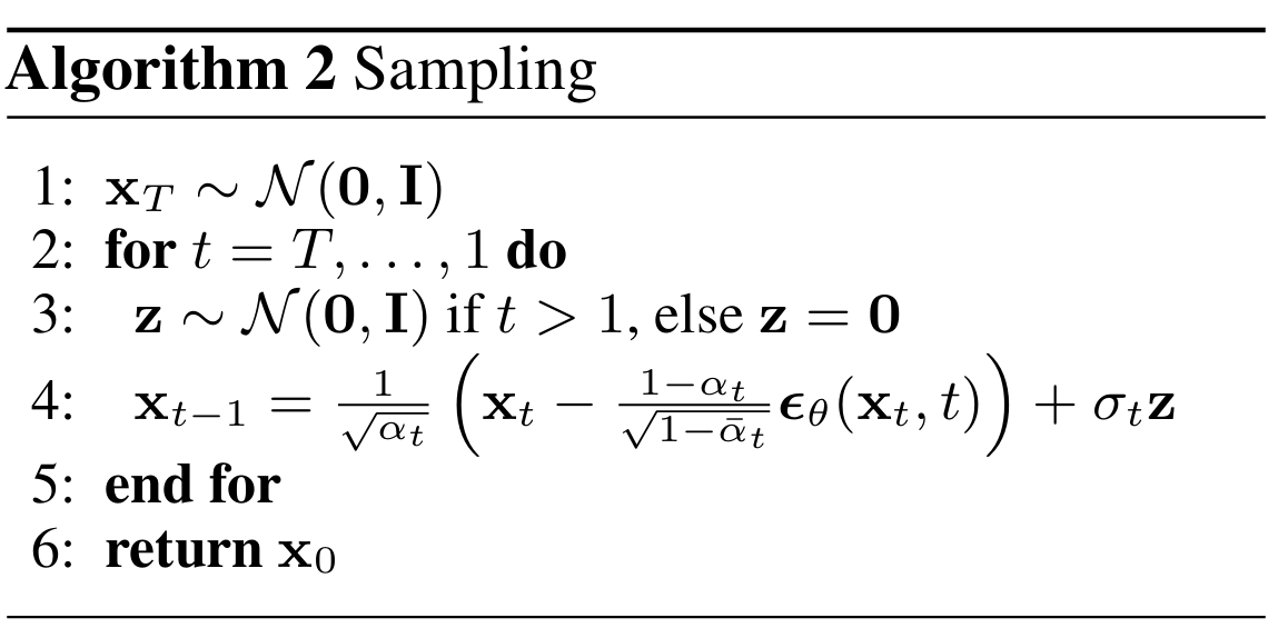
这是生成阶段的伪代码,同样也很简单:
如果你仔细看这个伪代码就会发现,我们似乎在采样过程也加入了噪声(就是伪代码里的 \(z\) )。可是,我们明明不是都要生成图像了吗?为什么还要在每一步去噪的同时加入噪声呢?
我们知道,反向过程一般写成一个高斯分布:
\[
p_\theta(x_{t-1}\mid x_t) = \mathcal{N}(\mu_\theta(x_t,t), \Sigma_\theta(x_t,t))
\]
这是一个概率分布。这意味着,从 \(x_t\) 到 \(x_{t-1}\) 的过程不仅有一个均值,还会有一定随机性。所以,为了体现这种随机性,在采样时,我们往往会按照模型给出的均值方向前进的同时,再加入一点随机扰动。也就是说,每一步采样的过程是:
\[
x_{t-1} = \mu_\theta(x_t, t) + \sigma_\theta(x_t, t) \cdot z
\]
如果完全没有随机性,采样路径可能会过于僵硬。适当保留一些随机扰动,则更符合原始概率模型的定义。也就是说,DDPM 的采样过程本质上也是一个随机过程,而不是一个完全确定的过程。
当然,后来也有很多变体(例如 DDIM)把 DDPM 的随机采样过程改写成了一个可以是确定性的更新过程。但在最基础的 DDPM 里,逐步采样 + 每步带一点随机性 是标准做法。
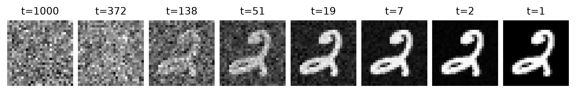
= dnnlpy.get_data_root()= v2.Compose([v2.ToImage(), v2.ToDtype(torch.float32, scale= True )])= datasets.MNIST(root, train= False , download= True , transform= transform)= random.randrange(len (ds))= ds[idx][0 ].squeeze(0 ) # shape: (28, 28) def denoise_v2(x0: Tensor, xt: Tensor, timestep: int , betas: Tensor) -> Tensor:= timestep= 1.0 - betas= alphas[t]= alphas.cumprod(dim= 0 )= alpha_bars[t]= alpha_bars[t - 1 ] if t > 0 else torch.tensor(1.0 )= betas[t]= alpha_bar_prev_t.sqrt() * beta_t / (1 - alpha_bar_t)= alpha_t.sqrt() * (1 - alpha_bar_prev_t) / (1 - alpha_bar_t)= param1 * x0 + param2 * xt= (1 - alpha_bar_prev_t) / (1 - alpha_bar_t) * beta_tif t > 0 :# Add noise for all steps except the last one = torch.randn_like(x0)return mean + variance.sqrt() * zelse :return mean= 1000 = torch.linspace(0.0001 , 0.02 , steps= T)= ddpm.add_noise(x0, betas, T - 1 )= [xt.clone()]for t in range (T - 1 , - 1 , - 1 ):= denoise_v2(x0, xt, t, betas)# We use step=8 here for better visualization = torch.logspace(3 , 0 , steps= 8 , dtype= torch.long )= [trajectory[T - i] for i in idx - 1 ]= plt.figure(2 , figsize= (8 , 2 ))= fig.subplots(1 , len (trajectory))for i, ax in enumerate (axes):= 'gray' )'off' )f't= { idx[i]} ' , fontsize= 10 )= 0.5 )'highdpi' )
14.4.5 DDPM 训练与采样的简化代码
到这里,我们可以把整个 DDPM 的实现流程用 PyTorch 代码写出来。为了方便后面引入 Hugging Face diffusers 库,这里的 API 与 diffusers 的设计保持一致。
14.4.5.1 训练过程
训练过程主要分为以下几个步骤:
从数据集中采样一个真实图像 \(x_0\) ;
随机采样一个时间步 \(t\) ;
从高斯分布中采样一个噪声 \(\epsilon\) ;
根据前向过程公式,构造带噪图像 \(x_t\) ;
把 \(x_t\) 和 \(t\) 输入模型,得到噪声预测 \(\hat{\epsilon}\) ;
计算损失,更新模型参数。
这里的 add_noise() 函数就是我们在前几节定义的 add_noise_v2() 函数。它根据前向过程闭式公式,把 \(x_0\) 和 \(\epsilon\) 结合起来,根据任意时间步 \(t\) 直接构造出 \(x_t\) 。add_noise() 函数同时额外添加了对于 batch 维度的支持,以便在实际训练中处理批量数据,从而提高训练效率。
= torch.randn(32 , 3 , 32 , 32 )= utils.TensorDataset(data)= utils.DataLoader(train_ds, batch_size= 16 , shuffle= True )= UNet2DModel().to(device)= DDPMScheduler()# 1. Iterate over the training data. for x0, * _ in train_dl:= x0.to(device) # [B, C, H, W] # 2. Sample random time steps for each image in the batch. = torch.randint(0 ),),= torch.long ,= device,# 3. Sample noise to add to the images. = torch.randn_like(x0)# 4. Add noise to the clean images according to the sampled time steps. = scheduler.add_noise(x0, noise, timesteps)# 5. Predict the noise using the model. = model(xt, timesteps)# 6. Compute the loss between the predicted noise and the actual noise. = F.mse_loss(pred_noise, noise)print ('Training step completed, loss:' , loss.item())
Training step completed, loss: 1.0702728033065796
14.4.5.2 采样过程
采样过程主要分为以下几个步骤:
从标准正态分布中采样一个噪声图像 \(x_T\) ;
设置时间步序列,例如 \(T, T-1, \dots, 1\) ;
对于每一个时间步 \(t\) ,构造一个全是 \(t\) 的批次向量 \(t_{batch}\) ;
对于当前的 \(x_t\) 和 \(t_{batch}\) ,输入模型得到噪声预测 \(\hat{\epsilon}\) ;
根据反向过程公式,计算 \(x_{t-1}\) ,可能还要加上随机扰动;
最终得到 \(x_0\) ,即生成的图像。
这里的 step() 函数就是我们在前几节定义的 denoise_v2() 函数。它根据反向过程公式,计算出 \(x_{t-1}\) 的均值和方差,并根据当前去噪步数是否是最后一步来决定是否加入随机扰动。step() 函数同时额外添加了对于 batch 维度的支持,以便在实际采样过程中处理批量数据,从而提高采样效率。
# 1. Start from pure noise (e.g., a random tensor). = torch.randn(1 , 3 , 32 , 32 , device= device)# 2. Set the number of inference timesteps. # Usually less than the number of training timesteps, e.g., 100. 100 , device= device)eval ()with torch.inference_mode():for t in scheduler.timesteps:# 3. Construct a batch of time steps (same time step for the whole batch). = torch.full((xt.size(0 ),), int (t), dtype= torch.long , device= device)# 4. Predict the noise using the model. = model(xt, t_batch)# 5. Compute the previous sample using the scheduler's step function. = scheduler.step(pred_noise, int (t), xt)# 6. The final sample after the last time step is the generated image. print (xt.shape)
torch.Size([1, 3, 32, 32])
其实从采样过程也不难发现,为什么 DDPM 的采样通常比较慢了。因为它不是一步生成,而是要跑很多步,每一步都要做一次 U-Net 前向传播,所以整体生成成本会比较高。但是,也正是因为这个逐步的过程,DDPM 才能生成质量非常高的图像。
14.4.6 本章小结
这一节我们从实现角度看了 DDPM 的网络结构与采样过程。可以把它概括成下面几句话:
DDPM 的网络并不是直接生成图像,而是在每一步预测噪声;
模型必须知道当前时间步,因此时间 embedding 是关键组成部分;
U-Net 很适合这种像素级、条件式、多尺度的去噪任务;
采样时从纯噪声开始,重复调用同一个去噪网络,一步一步得到最终图像。
到这里,DDPM 的怎么做已经基本完整了。但是,到目前为止,我们还没有真正从概率建模的角度去理解它。DDPM 的训练目标只是工程上的经验技巧吗?还是说,它其实能从一个严格的概率模型目标推导出来?
下一节,我们会重新回到概率建模的视角,看看 DDPM 的目标函数到底是怎么从 ELBO 一步一步推出来的,以及为什么最后会化简成我们现在看到的噪声预测损失。