1.5 Why Neural Networks Can Be Trained: Optimization Intuition in High-Dimensional Spaces

In the previous sections, we broke down the training process of a neural network step by step. The model first obtains a prediction through the forward pass, then uses a loss function to measure the gap between the prediction and the target; backpropagation computes the gradients, and gradient descent updates the parameters according to those gradients. Thus, one basic training step can be written as:
\[ \text{Forward} \rightarrow \text{Loss} \rightarrow \text{Backward} \rightarrow \text{Update} \]
From a procedural perspective, this seems to explain everything. But if we think more deeply, we find a stranger question:
Why does this approach actually manage to train neural networks?
A modern neural network may have millions, billions, or even more parameters. Its loss function \(L(\theta)\) is defined over an extremely high-dimensional parameter space and is usually a complex non-convex function. Based on the intuition we form from two-dimensional images, such a function should be full of peaks, valleys, and local minima. Gradient descent sees only the gradient near its current position at each step; it cannot see the entire loss function or know where the global optimum is. Why, then, does it not fall into some small pit after a few steps and get stuck there forever?
Furthermore, the number of parameters in a neural network is often large enough to memorize the training data. If the model has so many degrees of freedom, why can it not only reduce the training loss, but also often work on data it has never seen?
There is still no simple, unified answer to these questions today. Deep-learning theory continues to study the relationship among optimization, representation learning, and generalization. However, we already know some important intuitions. They help us understand that although a neural network is a huge non-convex optimization problem, it is not as hopeless as a two-dimensional image might suggest.
1.5.1 The Loss Landscape Is Not a Two-Dimensional Valley Map
We often draw gradient descent as a small ball rolling downward along a curve:
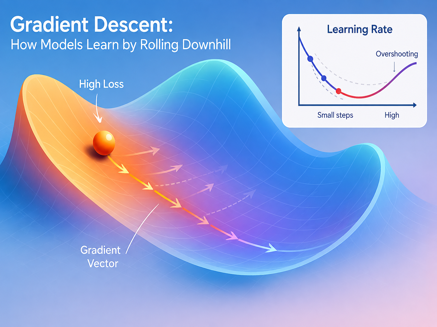
This picture is useful, but it can easily create a mistaken intuition: it may seem that training a neural network means searching for the lowest point on a rippled curve or surface. The actual situation is completely different.
If a model has \(d\) parameters, we can write all its parameters as a vector:
\[ \theta = (\theta_1, \theta_2, \ldots, \theta_d) \]
The loss function is:
\[ L:\mathbb{R}^d \rightarrow \mathbb{R} \]
In other words, every parameter configuration corresponds to a point in parameter space, and the height of that point is the current loss. If the model has one billion parameters, this space is one billion-dimensional. The two-dimensional loss landscapes we usually see can only be a slice or projection of this enormous space, not the complete loss function.
Therefore, one of the most important principles in high-dimensional optimization is: do not directly transfer the intuition of a two-dimensional terrain map to high-dimensional space.
For example, in a one-dimensional function, if we reach a point where the gradient is zero, we usually only need to determine whether it is the top of a hill or the bottom of a valley. But in high-dimensional space, a zero gradient only means:
\[ \nabla L(\theta) = 0 \]
Yes, it only tells us that the gradient is 0 at this point; it does not tell us what kind of point it is. Therefore, we must also examine the curvature in different directions. These local curvatures can be described by the Hessian matrix:
\[ H = \nabla^2 L(\theta) \]
If we decompose the Hessian into different directions, we obtain a set of eigenvalues:
\[ \lambda_1,\lambda_2,\ldots,\lambda_d \]
They can be roughly understood as indicating whether the loss function curves upward or downward when we move from the current position along different directions.
| Critical point | Typical Hessian condition | Intuition |
|---|---|---|
| Local minimum | Curves upward in every direction | The loss increases no matter which direction we move |
| Local maximum | Curves downward in every direction | The loss decreases no matter which direction we move |
| Saddle point | Curves upward in some directions and downward in others | Some directions look like the bottom of a valley, but other directions still allow descent |
A saddle point in two-dimensional space can be imagined as a horse saddle: viewed along one direction, it looks like a low point; viewed along another, it looks like a high point.
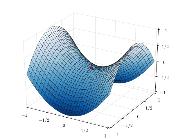
When the parameter dimension is extremely high, a critical point must have no descent direction in every direction before it can be a strict local minimum. As long as there is a direction with negative curvature, there is still a direction in which we can leave.
This is why researchers noticed early in the study of high-dimensional non-convex optimization that the places that truly slow optimization are not necessarily just “bad local minima”. Large numbers of saddle points and flat regions are equally important. An optimizer may arrive at a point where the gradient is already very small and appear to stop moving, but this does not mean it has entered a true local minimum.
However, we must be especially careful here. We cannot conclude from this that:
Because the parameter dimension is high, neural networks will not encounter local minima.
This conclusion is too strong. The loss landscape of a real neural network has a highly complex structure and is not a randomly generated high-dimensional function. High-dimensional geometry can help us understand why “being full of bad, isolated little pits” is not the only reasonable picture, but it cannot guarantee that gradient descent will find the global optimum.
1.5.2 Overparameterization: We May Not Need to Find a Unique Answer at All
There is another highly counterintuitive phenomenon: neural networks have many parameters, which sounds as though it should make optimization more difficult, but in modern deep learning, more parameters often make training easier instead.
To understand this, first consider a very simple problem. Suppose we have only two parameters, \(\theta_1\) and \(\theta_2\), but the training data requires them to satisfy three mutually independent conditions. These three conditions may simply be impossible to satisfy simultaneously:
\[ \begin{align} f_1(\theta_1,\theta_2) &= 0,\\ f_2(\theta_1,\theta_2) &= 0,\\ f_3(\theta_1,\theta_2) &= 0, \end{align} \]
There are too few degrees of freedom, so we can only compromise among the conditions. Conversely, if we have many parameters but need to satisfy relatively few constraints, the parameter configurations satisfying those constraints may no longer be a single point, but an entire region.
The simplest linear example is:
\[ \theta_1 + \theta_2 = 1 \]
It does not have only one solution, but infinitely many:
\[ (0,1),\quad (0.2,0.8),\quad (2,-1),\quad \ldots \]
All the solutions together form a straight line.
Neural networks are of course much more complex than this example, but the intuition from overparameterization is similar: when a model has many degrees of freedom, there may be very many parameter configurations that fit the training data well. The optimizer does not necessarily need to find the one unique “correct answer” in the entire parameter space; it only needs to enter a sufficiently good solution region.
Therefore, neural-network training is not searching for the single lowest point in a huge mountain range. It is closer to this:
There are many low-loss positions in parameter space, perhaps even continuous low-loss regions, and we only need to find one of them.
There is another reason that makes the concept of a “unique optimal parameter” less important: neural networks have parameter symmetries.
For example, suppose two neurons in a hidden layer perform the same function. If we swap the order of these two neurons and simultaneously swap the corresponding connections in the next layer, the function computed by the entire network can remain exactly unchanged. That is:
\[ \theta_a \neq \theta_b \]
but it may still be that:
\[ f(x;\theta_a) = f(x;\theta_b) \]
Therefore, even considering exactly the same function, there may be many different parameter representations. The goal of training a neural network has never been to recover one unique set of “true parameters,” but to find a set of parameters that implements the function behavior we need.
This is an important shift in how to understand modern deep-learning optimization:
Having more parameters is not only a burden; it also gives the optimization process more degrees of freedom and more feasible paths.
Of course, overparameterization is not a theorem saying that more parameters are always better. Increasing the size of a model also brings greater computational, memory, and data requirements, and the optimization properties of different architectures vary. Here, we only need to grasp one central intuition: in deep learning, a huge parameter space does not mean that good solutions are rarer; in many cases, quite the opposite is true, and good solutions may be abundant.
1.5.3 Why Does SGD Not Easily Stop Just Anywhere?
The previous discussion concerned the geometry of the loss landscape. Next, let us look at the actual training algorithm.
If we use the complete dataset to compute the gradient, gradient descent obtains:
\[ g = \nabla_\theta L(\theta) \]
But when training neural networks in practice, we almost always use a mini-batch. Suppose the current batch is \(B\); then we compute:
\[ g_B = \nabla_\theta \frac{1}{|B|} \sum_{i\in B} L_i(\theta) \]
Different batches contain different data, so usually:
\[ g_B \neq \nabla_\theta L(\theta) \]
In other words, the gradient seen by SGD is not an exactly precise descent direction on the full loss landscape, but a stochastic estimate. Therefore, the actual training trajectory is not like a small ball smoothly rolling downhill along the steepest direction. It is more like “an overall downward trend + continuous random jitter.”
At first, this randomness may look like a drawback because each step is less accurate. But it can sometimes help optimization instead. For example, near a very flat region, the full gradient may already be very small, while the gradients produced by different mini-batches may still fluctuate; near some saddle points with descent directions, these perturbations may also help the parameters leave the current region.
Again, however, we cannot state this conclusion too absolutely. The noise in SGD does not guarantee that the model will escape every saddle point, much less that it will find the global optimum. The learning rate, batch size, momentum, parameter initialization method, and network architecture all change the optimization process. We will gradually see these factors in the later chapter on optimization algorithms. What is genuinely worth remembering is:
Training a neural network is not a deterministic ball mechanically rolling on a fixed surface. It is a high-dimensional, stochastic, dynamic process continually influenced by both the data and the optimizer.
This is also why two otherwise identical models can end up with completely different parameters even when they use the same data, as long as their random initializations or mini-batch orders differ. Yet the functions they ultimately implement may be equally good.
1.5.4 The Data May Be High-Dimensional, but It May Not Be as Complex as It Looks
So far, we have been discussing parameter space. But the ability of neural networks to learn is also related to another space: the space in which the input data lies.
For example, an RGB image of size \(224\times 224\) contains:
\[ 224\times 224\times 3 = 150528 \]
values. Formally, every image is a point in \(\mathbb{R}^{150528}\).
How large is this space? If every pixel could vary independently and arbitrarily, nearly all possible points would look like random noise. Real natural images occupy only a tiny fraction of the entire pixel space. The faces, animals, street scenes, and text we see are not arbitrary combinations of pixels. They are constrained by substantial structure in the real world: objects have continuous contours, neighboring pixels are highly correlated, lighting changes are usually continuous, and an object remains the same object after a small rotation.
This leads to an influential intuition in machine learning: the Manifold Hypothesis. It states:
Although real-world data is represented in a very high-dimensional space, useful data is often concentrated near a structure with much lower dimensionality.
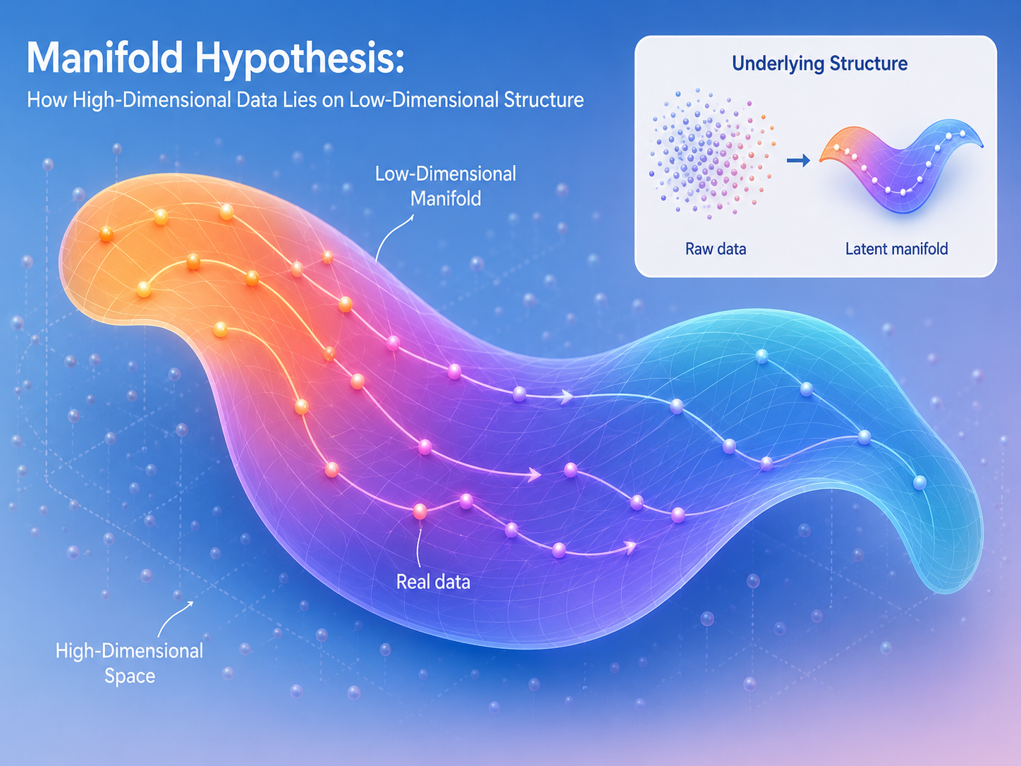
If this intuition holds for a task, the model does not actually need to learn how to handle every possible point in the high-dimensional input space. It mainly needs to learn the correct mapping in the small region where real data commonly occurs. This makes “learning a high-dimensional function” less frightening than it appears on the surface.
For example, an image-classification model does not need to know what every 150528-dimensional random vector means. It only needs to form useful decision boundaries near natural images. The successive representation transformations inside a neural network can also be understood as continually reorganizing the input into representation spaces better suited to the current task:
\[ x \rightarrow h_1 \rightarrow h_2 \rightarrow \cdots \rightarrow h_L \]
For classification tasks, we hope these transformations make originally entangled data easier to distinguish; for generation tasks, we hope the model can capture the stable, structured patterns of variation in real data.
However, we must clearly distinguish two concepts that are easy to confuse. The overparameterization discussion above concerns the possibility that solutions in parameter space may form a continuous structure; the Manifold Hypothesis here concerns the possibility that real data in input space may be concentrated near a low-dimensional structure. They may both involve the word “manifold,” but they refer to two entirely different things.
Moreover, the Manifold Hypothesis is not a theorem that has been rigorously proved for all real-world data. Real data usually contains discrete structures, noise, multi-scale variation, and complex topology; describing all data with one smooth low-dimensional manifold is often too idealized. It is more accurate to understand it as a hypothesis that helps us think about why high-dimensional data may still have learnable structure. More importantly, low-dimensional data structure cannot by itself prove that neural-network optimization is easy. The structure of input space addresses “why the task may contain regularities,” while the geometry and optimization dynamics of parameter space address “why we may find parameters that implement those regularities.” These two questions are related, but they must not be conflated.
1.5.5 Reducing the Loss Is Not Even the Most Amazing Part
At this point, we can give a less mysterious answer to the question we started with. Neural networks can be trained because several factors work together:

First, neural networks consist of many continuous, almost-everywhere differentiable operations, so backpropagation can efficiently provide local gradients. Although a gradient cannot see the entire parameter space, it can continually provide a direction for improvement near the current position.
Second, high-dimensional non-convex spaces are not simply filled with isolated little pits. Saddle points, flat directions, and complex low-loss regions are also abundant, so the two-dimensional intuition that “gradient descent will necessarily fall quickly into a bad local minimum” is unreliable.
Finally, modern neural networks are usually highly overparameterized. Models have many degrees of freedom, so there may be many parameter configurations that complete the training task, and the optimizer often does not need to find one unique, exact answer. At the same time, the randomness brought by mini-batches prevents the SGD trajectory from moving entirely along one fixed direction, while real data itself has substantial structure, so the model is not facing a completely arbitrary high-dimensional mapping problem.
But if we look carefully, we find that we have actually answered only one question:
Why can the training loss be optimized?
The truly more surprising question in deep learning is another one:
Why can a trained neural network generalize?
A network whose number of parameters greatly exceeds the number of training examples often has enough capacity to simply memorize the training data. If our only goal were to reduce the training loss, overparameterization would indeed provide substantial help. But why can a model often make correct predictions on data it has never seen while fitting the training set extremely well? This cannot be explained merely by saying that “gradient descent found a low-loss solution.”
Optimization tells us how to find a solution in parameter space, while generalization asks:
Why does the solution we find happen to be useful for data outside the training set as well?
The data distribution, the inductive bias of the network architecture, the implicit bias of the optimizer, regularization, data augmentation, and model scale all play a role. This is one of the most interesting aspects of modern deep-learning theory. The fact that neural networks can be trained does not mean that we fully understand why they work.
1.5.6 Summary
This section did not introduce any new training step. Instead, it took a step back and discussed a more fundamental question: since a neural network is a huge non-convex optimization problem, why can gradient-based methods still train it?
First, we cannot directly imagine the real loss landscape as a two-dimensional valley map. The parameter space of a neural network may have millions or even billions of dimensions. A point where the gradient is close to zero is not necessarily a local minimum; it may also be a saddle point or an extremely flat region. There are many different directions in high-dimensional space, so “the optimizer will be trapped everywhere by bad local minima” is not an accurate enough description.
Second, modern neural networks are usually overparameterized. Having many parameters does not only mean a larger search space; it also gives the model more degrees of freedom. Solutions that fit the training data well are often not unique, so the optimizer may not need to search for an isolated optimum and may only need to enter one of many low-loss solutions.
The randomness of SGD also changes the optimization trajectory. The mini-batch gradient is a noisy estimate of the full gradient, and these perturbations can sometimes help the model leave flat regions or saddle points with descent directions. However, this does not guarantee that training will succeed, nor that it will find the global optimum.
Finally, we saw another important intuition from the input space. Although real data is represented in a high-dimensional space, it usually has substantial internal structure. The Manifold Hypothesis attempts to describe this phenomenon as “a low-dimensional structure in a high-dimensional space.” However, the data manifold and the structure of solutions in parameter space are two different concepts, and low-dimensional data structure alone cannot directly prove that optimization is easy.
Therefore, neural networks can be trained not because one magical theorem guarantees that gradient descent will always succeed, but because many factors make the problem friendlier than it appears: the network is differentiable, the gradients contain information, high-dimensional space has many directions, overparameterization provides abundant feasible solutions, SGD is stochastic, and real data is not structureless.
At this point, we have completed the most important task of Chapter 1: starting from the idea that a neural network is a learnable function, we have seen step by step how a model defines error, computes gradients, and updates parameters, as well as why such an apparently unbelievable high-dimensional optimization process can genuinely work in practice.
Next, we will move on to PyTorch and see how these abstract concepts are implemented in a real deep-learning framework.