In the previous sections, we have seen that basic SGD has two important problems.
The first problem is that mini-batch SGD is noisy. If each step only looks at the gradient of the current batch, the update direction may fluctuate, especially in the early stage of training, when the model has not yet learned many useful features.
Momentum improves this by not looking only at the current gradient. Instead, it maintains a moving average of historical gradient directions:
\[
m_t = \beta m_{t-1} + (1 - \beta) g_t
\]
In this way, the update direction is no longer completely determined by the current batch. It carries a certain amount of inertia.
The second problem is that different parameters may have very different gradient scales. If all parameters share the same learning rate, some parameters may update too quickly, while others may update too slowly.
RMSProp improves this by maintaining a moving average of squared gradients for each parameter:
\[
v_t = \rho v_{t-1} + (1 - \rho) g_t^2
\]
Then it uses \(\sqrt{v_t}\) to scale the current gradient:
In this way, parameters whose gradients have been large for a long time will have their step sizes reduced, while parameters whose gradients have been small for a long time can keep relatively larger step sizes.
At this point, a natural question is:
Can we combine Momentum and RMSprop?
In other words, we want the update direction not to be completely controlled by the noise of the current batch, while also allowing each parameter to have an adaptive learning rate.
This is the core idea of Adam (Adaptive Moment Estimation)(Kingma and Ba 2017).
from collections.abc import Iterablefrom typing import overrideimport dnnlpyimport dnnlpy.optim as doptimport matplotlib.pyplot as pltimport torchimport torch.nn as nnimport torch.nn.functional as Ffrom torch import Tensordnnlpy.set_matplotlib_format('svg')print('PyTorch version:', torch.__version__)
PyTorch version: 2.14.0+cpu
4.5.1 Adam Tries to Solve Two Problems at the Same Time
To understand where Adam fits, let us first put the previous optimizers together.
The update rule of SGD is:
\[
\theta_{t+1} = \theta_t - \eta g_t
\]
It only uses the current gradient \(g_t\).
Momentum first maintains the first moment:
\[
m_t = \beta m_{t-1} + (1 - \beta) g_t
\]
Then it uses \(m_t\) to update the parameters:
\[
\theta_{t+1} = \theta_t - \eta m_t
\]
Here, \(m_t\) can be understood as a moving average of gradient directions. It solves the problem of directional fluctuation.
RMSprop maintains a moving average of squared gradients:
\[
v_t = \rho v_{t-1} + (1 - \rho) g_t^2
\]
Then it uses this quantity to scale the current gradient:
Here, \(v_t\) can be understood as the gradient scale over a recent period of time. It solves the problem of different gradient scales across parameters.
Adam puts these two ideas together. It maintains two states at the same time:
That is, the numerator determines the update direction, while the denominator determines the scaling for each parameter.
4.5.2 First Moment: Smoothing the Gradient Direction
Adam’s first state is \(m_t\):
\[
m_t = \beta_1 m_{t-1} + (1 - \beta_1) g_t
\]
This formula is very similar to momentum. It does not directly use the current gradient \(g_t\). Instead, it mixes the current gradient with the past momentum. If \(\beta_1\) is large, the past direction contributes more, and the update direction becomes smoother. If \(\beta_1\) is smaller, the current gradient has a stronger influence, and the update direction becomes more responsive.
A commonly used default value in Adam is:
\[
\beta_1 = 0.9
\]
This means that the current gradient only contributes 0.1, while the past momentum contributes 0.9. In other words, Adam will not immediately change the update direction dramatically just because the gradient of one mini-batch suddenly changes.
Intuitively, \(m_t\) answers this question:
Over the recent past, where have the gradients roughly been pointing?
SGD only cares about the gradient of the current batch at each step. Adam’s first moment, however, cares about the average direction over a recent period of time. This is the part that Adam inherits from momentum.
4.5.3 Second Moment: Estimating the Gradient Scale of Each Parameter
Adam’s second state is \(v_t\):
\[
v_t = \beta_2 v_{t-1} + (1 - \beta_2) g_t^2
\]
The square here is element-wise. In other words, each parameter has its own \(v_t\).
If a parameter has had large gradients for a long time, its corresponding \(v_t\) will become large. During the update, the denominator becomes larger, so the effective step size of this parameter becomes smaller. If a parameter has had small gradients for a long time, its corresponding \(v_t\) will be smaller. During the update, the denominator is smaller, so this parameter can still have a relatively large effective step size.
A commonly used default value in Adam is:
\[
\beta_2 = 0.999
\]
This value is usually closer to 1 than \(\beta_1\), which means the second-moment estimate has a longer memory. The reason is also intuitive: the gradient direction may need to adapt more quickly to the current batch, but the gradient scale is usually something we want to estimate more stably.
Intuitively, \(v_t\) answers this question:
Over the recent past, how large has the gradient of each parameter been?
Therefore, Adam’s two states correspond to two questions:
\(m_t\): What is the direction?
\(v_t\): How large is the scale?
In the final update, Adam uses \(m_t\) as the direction and uses \(\sqrt{v_t}\) for scaling.
4.5.4 Why Do We Need Bias Correction?
If Adam only combined momentum and RMSProp, the two formulas below might seem to be the end of the story:
However, Adam is not an absolutely better optimizer. It introduces more states and more hyperparameters. More importantly, the way Adam combines with weight decay also causes a problem, which leads to the next section on AdamW.
4.5.5 PyTorch Implementation of Adam
Next, let us implement a simplified version of Adam in PyTorch.
class Adam(dopt.Optimizer):def__init__(self, params: Iterable[Tensor], lr: float=1e-3, betas: tuple[float, float] = (0.9, 0.999), eps: float=1e-8, weight_decay: float=0.0, ):super().__init__(params)self.lr = lrself.beta1 = betas[0]self.beta2 = betas[1]self.eps = epsself.weight_decay = weight_decayself.step_count =0self.exp_avg = [torch.zeros_like(p) for p inself.params]self.exp_avg_sq = [torch.zeros_like(p) for p inself.params]@override@torch.no_grad()def step(self):self.step_count +=1for p, m, v inzip(self.params,self.exp_avg,self.exp_avg_sq, strict=True, ):if p.grad isNone:continue grad = p.gradifself.weight_decay >0: grad = grad.add(p, alpha=self.weight_decay) m.mul_(self.beta1).add_(grad, alpha=1-self.beta1) v.mul_(self.beta2).addcmul_(grad, grad, value=1-self.beta2) bias_correction1 =1-pow(self.beta1, self.step_count) bias_correction2 =1-pow(self.beta2, self.step_count) m_hat = m / bias_correction1 v_hat = v / bias_correction2 p.addcdiv_(m_hat, v_hat.sqrt() +self.eps, value=-self.lr)
There are several states to pay attention to here.
exp_avg corresponds to \(m_t\) in the formula, namely the first moment. exp_avg_sq corresponds to \(v_t\) in the formula, namely the moving average of squared gradients. step_count is used to compute \(1 - \beta_1^t\) and \(1 - \beta_2^t\) in bias correction.
As before, zero_grad() clears the .grad attribute of the parameters, not Adam’s internal states. Adam’s exp_avg and exp_avg_sq must be preserved across steps; otherwise, there would be no “momentum” or “moving average”.
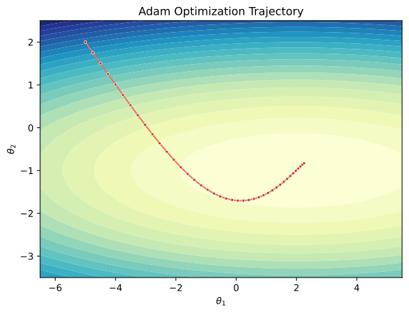
We can use a simple linear regression task to check whether our Adam implementation can train normally.
We can see that our Adam implementation successfully optimizes this simple quadratic function, and the parameters gradually converge to the optimum \((2, -1)\).
4.5.6 Why Is Adam Commonly Used?
Adam is very common in deep learning, not because it is theoretically optimal in all cases, but because it has several practical advantages.
First, Adam is relatively less sensitive to the learning rate. SGD often requires careful tuning of the learning rate and the learning-rate schedule. Because Adam has adaptive scaling, many tasks can start training with the default parameters.
Second, Adam can handle cases where different parameters have very different gradient scales. The gradient distributions of different layers and parameters in a neural network may vary greatly. Adam’s second-moment scaling can automatically adjust the effective step size of each parameter.
Third, Adam’s first moment can reduce mini-batch gradient noise, making the update direction smoother than ordinary SGD.
These properties make Adam a strong baseline optimizer for many tasks. Especially in training scenarios that are relatively complex, such as Transformers, generative models, and reinforcement learning, Adam or AdamW is often the default choice.
However, Adam also has costs.
It needs to maintain two extra states for each parameter: \(m_t\) and \(v_t\). If the model has \(P\) parameters, Adam needs to store roughly an additional \(2P\) states. This increases GPU memory or system memory usage. In addition, Adam’s adaptive learning rate may sometimes affect generalization. In some vision fine-tuning tasks, SGD with momentum may achieve better results.
Therefore, if our goal is to get the model training quickly, Adam is a good choice. If we care more about generalization performance, or if the model is relatively small, SGD with momentum may be more suitable.
4.5.7 What Is Adam Still Missing?
At this point, Adam seems quite complete:
It uses the first moment to smooth the gradient direction;
It uses the second-moment estimate to scale the update of each parameter;
It uses bias correction to correct the early-stage bias in training.
Then why do we still need to discuss AdamW in the next section?
The reason is not that the algorithm is incomplete, but that there is a problem with how Adam combines with weight decay.
First consider SGD. Suppose we add an L2 regularization term to the loss:
This formula is easy to understand: besides the normal gradient descent step, each step also multiplies the parameters by a coefficient smaller than 1, namely \((1 - \eta\lambda)\). Therefore, the parameters are gently pulled toward 0. This is weight decay.
In SGD, adding the L2 regularization term to the gradient and directly applying weight decay are basically the same thing. But in Adam, this is different. Adam does not directly use \(g_t\) to update the parameters. Instead, it first puts the gradient into the first moment and the second moment:
If we add the L2 regularization term directly to the gradient as in SGD:
\[
g_t \leftarrow g_t + \lambda \theta_t
\]
then \(\lambda \theta_t\) will also enter Adam’s \(m_t\) and \(v_t\), and it will eventually be scaled by \(\sqrt{\hat{v}_t} + \epsilon\). As a result, weight decay is no longer simply pulling the parameters toward 0. How much a parameter is pulled toward 0 also depends on the past gradient scale of that parameter.
This is somewhat strange. Weight decay is supposed to care about the parameter magnitude, and it should not be reinterpreted by Adam’s adaptive learning rate.
That is, AdamW does not replace Adam. It separates two things:
Adam is responsible for descending according to the gradient;
Weight decay is responsible for independently shrinking the parameters.
Therefore, in modern deep learning, especially for models such as Transformers, ViTs, and LLMs, AdamW is usually used more often than ordinary Adam with weight decay. The core reason is that the meaning of weight decay in AdamW is cleaner and easier to tune.
4.5.8 Summary
In this section, we introduced Adam.
Adam can be understood as a combination of momentum and RMSProp. It maintains the first moment \(m_t\) to smooth the gradient direction, and it also maintains the second moment \(v_t\) to estimate the gradient scale of each parameter. In the final update, Adam uses the first moment as the direction and uses the square root of the second moment to scale the effective learning rate of each parameter.
Since both \(m_t\) and \(v_t\) are initialized from 0, they are biased toward 0 in the early stage of training. Therefore, Adam also uses bias correction:
Adam’s advantages are that training is usually relatively stable, it is less sensitive to the learning rate, and it can adapt to cases where different parameters have very different gradient scales. However, it needs to maintain extra first- and second-moment states, and it does not necessarily generalize better than SGD on all tasks. More importantly, there is a problem with how Adam combines with weight decay. In the next section, we will see that AdamW makes Adam more suitable for training modern deep learning models by decoupling weight decay from gradient updates.