4.4 RMSprop and Adadelta: Fixing Learning Rate Decay
Author
jshn9515
Published
2026-05-29
Modified
2026-06-05
In the previous section, we introduced Adagrad. Its core idea is: instead of letting all parameters share the same learning rate, maintain a historical accumulated squared gradient for each parameter:
\[
s_t = s_{t-1} + g_t^2
\]
Then use this accumulated quantity to scale the current gradient:
If a parameter often had large gradients in the past, its corresponding \(s_t\) will become larger, so its later effective learning rate will become smaller. If a parameter is rarely updated, its corresponding \(s_t\) grows more slowly, so it can still keep a relatively large effective learning rate later. This makes Adagrad very suitable for sparse features.
However, Adagrad also has an obvious problem: \(s_t\) only keeps growing, so the effective learning rate can only keep decreasing.
In other words, Adagrad has too long a memory. It sums all historical squared gradients since the beginning of training, regardless of whether gradients from a long time ago still represent the current optimization state. This causes a problem: in the later stages of training, the denominator may become very large, making the parameters almost stop updating.
So a natural question is:
Can we keep Adagrad’s idea of adaptive learning rates, but prevent the historical accumulator from growing without bound?
RMSprop (Tieleman and Hinton 2012) and Adadelta (Zeiler 2012) were both developed along this line of thinking. They no longer use the accumulated sum of all historical squared gradients. Instead, they use an exponential moving average (EMA) to record the gradient scale over a recent period.
from collections.abc import Iterablefrom typing import overrideimport dnnlpyimport dnnlpy.optim as doptimport matplotlib.pyplot as pltimport torchimport torch.nn as nnimport torch.nn.functional as Ffrom torch import Tensordnnlpy.set_matplotlib_format('svg')print('PyTorch version:', torch.__version__)
PyTorch version: 2.14.0+cpu
4.4.1 The Problem with Adagrad: Its Historical Memory Is Too Long
First, let us review Adagrad’s effective learning rate. Its update rule is:
This property is sometimes useful. For example, if a parameter is updated frequently, Adagrad will gradually reduce its step size and make training more stable. But the problem is that Adagrad does not forget gradients from a long time ago. Even if the model has already entered a new region, large gradients from the early stages will still remain inside \(s_t\) and continue to suppress the effective learning rate. As a result, training may become slower and slower in the later stages.
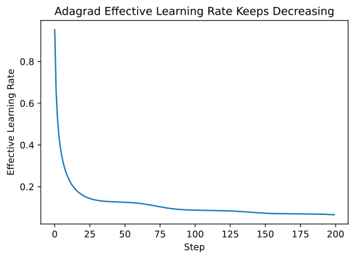
We can use a simple example to observe this phenomenon. Suppose the gradient magnitude of a parameter changes periodically. Adagrad’s historical accumulated squared gradient keeps increasing, so the effective learning rate keeps decreasing:
From the figure, we can see that even if the gradient magnitude at each step is periodic, Adagrad’s effective learning rate still keeps decreasing. This shows that the issue with Adagrad is not that it performs adaptive scaling, but that it uses the full historical accumulation from the beginning of training to the current time. If we want to fix this problem, we need another way to estimate the gradient scale.
4.4.2 From Accumulated Sum to Moving Average
Adagrad maintains the accumulated sum of historical squared gradients:
\[
s_t = s_{t-1} + g_t^2
\]
The problem with this formula is that all past gradients are permanently kept.
A natural modification is:
Do not accumulate the entire history. Instead, only keep the gradient scale over a recent period.
But we do not necessarily need to actually store all gradients from the most recent \(k\) steps. A more common approach is to use an exponential moving average:
\[
v_t = \rho v_{t-1} + (1 - \rho) g_t^2
\]
Here, \(\rho\) is usually a number close to 1, such as 0.9 or 0.99.
This formula can be understood as:
\(\rho v_{t-1}\): keep the previous estimate;
\((1 - \rho)g_t^2\): add information from the current squared gradient.
If \(\rho\) is large, more historical information is retained and the estimate changes more smoothly. If \(\rho\) is smaller, the current gradient has a larger influence and the estimate changes more quickly. The key difference is that the influence of old gradients decays exponentially over time.
For example, by expanding this recurrence, we get:
The older a gradient is, the smaller its weight becomes. This is like adding a forgetting mechanism to Adagrad: recent gradients matter more, while gradients from a long time ago slowly fade out.
4.4.3 RMSprop: Estimating Gradient Scale with a Moving Average
The core idea of RMSprop (Tieleman and Hinton 2012) is to replace Adagrad’s accumulated historical squared gradients with an exponential moving average of squared gradients.
Here, \(v_t\) can be understood as the recent average of the squared gradients for the current parameter. If a parameter has often had large gradients recently, \(v_t\) becomes larger, the denominator becomes larger, and the effective learning rate becomes smaller. This prevents the parameter from updating too aggressively. If a parameter has had small gradients recently, \(v_t\) becomes smaller, the denominator becomes smaller, and the effective learning rate becomes larger. This prevents the parameter from updating too slowly. Notice that the emphasis here is on recently.
This distinction from Adagrad is important.
Adagrad asks: how much squared gradient has this parameter accumulated since the beginning of training?
RMSprop asks: roughly what is the gradient scale of this parameter over a recent period?
Therefore, RMSprop is more suitable for non-stationary training processes.
Neural network training is inherently non-stationary. As parameters keep changing, the model also moves into different regions of the loss landscape. Gradient statistics from very early stages may no longer be suitable for the current region. By replacing full accumulation with a moving average, RMSprop allows the optimizer to gradually adapt to new gradient scales.
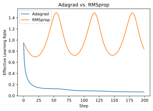
We can compare the effective learning rates of Adagrad and RMSprop side by side:
rho =0.9velocity = torch.tensor(0.0)rmsprop_lr_history = []for t, grad inenumerate(simulated_grad, start=1): velocity = rho * velocity + (1- rho) * grad.square()# We do bias correction to make it comparable to Adagrad's# effective learning rate. velocity_adj = velocity / (1-pow(rho, t)) lr = initial_lr / (velocity_adj.sqrt() + eps) rmsprop_lr_history.append(lr.item())fig = plt.figure(2, figsize=(6, 4))ax = fig.add_subplot(1, 1, 1)ax.plot(adagrad_lr_history)ax.plot(rmsprop_lr_history)ax.set_xlabel('Step')ax.set_ylabel('Effective Learning Rate')ax.legend(['Adagrad', 'RMSprop'])ax.set_title('Adagrad vs. RMSprop')plt.show()
In this example, we used a simple periodic gradient sequence. We can see that Adagrad’s effective learning rate keeps decreasing, while RMSprop’s effective learning rate fluctuates with changes in the gradient. This shows that RMSprop successfully avoids Adagrad’s learning rate decay problem through a moving average.
4.4.4 PyTorch Implementation of RMSprop
Below, we implement a simplified version of RMSprop. It needs to maintain a state called square_avgs, which records the moving average of squared gradients for each parameter.
class RMSprop(dopt.Optimizer):def__init__(self, params: Iterable[Tensor], lr: float=1e-2, rho: float=0.99, eps: float=1e-8, weight_decay: float=0.0, momentum: float=0.0, ):super().__init__(params)self.lr = lrself.rho = rhoself.eps = epsself.weight_decay = weight_decayself.momentum = momentumself.ema_of_sq_grads = [torch.zeros_like(p) for p inself.params]self.momentum_buffers = [torch.zeros_like(p) for p inself.params]@override@torch.no_grad()def step(self):for p, v, bufferinzip(self.params,self.ema_of_sq_grads,self.momentum_buffers, strict=True, ):if p.grad isNone:continue grad = p.gradifself.weight_decay >0: grad = grad.add(p, alpha=self.weight_decay) v.mul_(self.rho).add_(grad.square(), alpha=1-self.rho)ifself.momentum >0:buffer.mul_(self.momentum).addcdiv_(grad, v.sqrt() +self.eps) p.sub_(buffer, alpha=self.lr)else: p.addcdiv_(grad, v.sqrt() +self.eps, value=-self.lr)@torch.no_grad()def get_effective_lr(self) ->list[Tensor]: effective_lr = []for v inself.ema_of_sq_grads: lr =self.lr / (v.sqrt() +self.eps).clone() effective_lr.append(lr)return effective_lr
One thing to note is that zero_grad() clears the .grad attribute of the parameters, not RMSprop’s square_avgs. .grad is the gradient cache computed from the current mini-batch and should be cleared before each round of backpropagation. square_avgs is the optimizer’s internal state, used to record the moving average of historical squared gradients, and should be preserved across steps. This is the same as in Adagrad.
4.4.5 Adadelta: Reducing Dependence on the Learning Rate
RMSprop fixes Adagrad’s core problem: it replaces the accumulated sum of historical squared gradients with a moving average. But it still keeps a global learning rate \(\eta\):
This looks a little more complicated than RMSprop, but the intuition is not difficult.
RMSprop uses \(\sqrt{v_t}\) to estimate the recent gradient scale, then uses it to scale the gradient. Based on this, Adadelta asks another question: what was the scale of past parameter updates themselves? If past updates were large, this step can be relatively larger; if past updates were small, this step should also be relatively cautious.
The denominator comes from the recent gradient scale, and the numerator comes from the recent update scale.
This is also why Adadelta is often described as an optimizer that reduces dependence on the global learning rate. It tries to calibrate the scale of parameter updates using the scale of historical updates themselves. Therefore, in the original Adadelta, a global learning rate lr is not required. However, PyTorch’s Adadelta implementation still keeps an lr parameter. In other words, practical implementations usually still allow a global coefficient to further scale the update.
4.4.6 PyTorch Implementation of Adadelta
Below, we implement a simplified version of Adadelta. It needs to maintain two states:
square_avgs: the moving average of squared gradients;
accumulate_updates: the moving average of squared updates.
class Adadelta(dopt.Optimizer):def__init__(self, params: Iterable[Tensor], lr: float=1.0, rho: float=0.9, eps: float=1e-6, weight_decay: float=0.0, ):super().__init__(params)self.lr = lrself.rho = rhoself.eps = epsself.weight_decay = weight_decayself.ema_of_sq_grads = [torch.zeros_like(p) for p inself.params]self.ema_of_sq_updates = [torch.zeros_like(p) for p inself.params]@override@torch.no_grad()def step(self):for p, v, u inzip(self.params,self.ema_of_sq_grads,self.ema_of_sq_updates, strict=True, ):if p.grad isNone:continue grad = p.gradifself.weight_decay >0: grad = grad.add(p, alpha=self.weight_decay) v.mul_(self.rho).add_(grad.square(), alpha=1-self.rho) delta_x = (u +self.eps).sqrt() / (v +self.eps).sqrt() * grad u.mul_(self.rho).add_(delta_x.square(), alpha=1-self.rho) p.sub_(delta_x, alpha=self.lr)@torch.no_grad()def get_effective_lr(self) ->list[Tensor]: effective_lr = []for v, u inzip(self.ema_of_sq_grads,self.ema_of_sq_updates, strict=True, ): lr =self.lr * (u +self.eps).sqrt() / (v +self.eps).sqrt() effective_lr.append(lr)return effective_lr
The most important line in this code is:
delta_x = (u +self.eps).sqrt() / (v +self.eps).sqrt() * grad
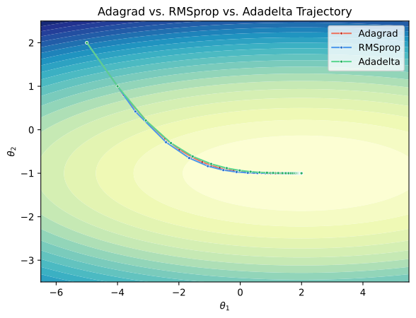
We can see that in this simple task, Adagrad accumulates the full history of squared gradients, so its effective learning rate keeps decreasing and the descent becomes noticeably slower in the later stage. In contrast, RMSprop and Adadelta both use exponential moving averages, so early gradients do not dominate later updates. However, on this task, the difference between their curves is not very obvious. The real differences are usually more visible on more complex tasks.
4.4.9 Summary
In this section, we started from the problem of Adagrad and introduced RMSprop and Adadelta.
Adagrad maintains an accumulated historical squared gradient for each parameter, thereby achieving adaptive learning rates. But this accumulator only increases and never decreases, causing the effective learning rate to keep decreasing. In the later stages of training, parameter updates may become very small.
RMSprop’s core improvement is to replace full historical accumulation with an exponential moving average. In this way, the influence of old gradients gradually decays, and the optimizer can adjust each parameter’s effective learning rate according to the gradient scale over a recent period.
Adadelta further introduces a moving average of squared historical updates. It uses the scale of past updates to calibrate the current update amount, attempting to reduce dependence on a manually chosen learning rate.
From the main line of optimizer evolution, RMSprop is especially important. This is because Adam can be understood as a combination of momentum and RMSprop: it maintains a first moment to smooth the gradient direction, and also maintains a second-moment estimate to scale each parameter’s update.
In the next section, we will introduce Adam from this perspective.
References
Tieleman, Tijmen, and Geoffrey Hinton. 2012. RMSprop: Divide the Gradient by a Running Average of Its Recent Magnitude.