In the previous sections, we implemented a two-layer MLP from scratch with NumPy:
\[
X
\rightarrow
\operatorname{Linear}
\rightarrow
\operatorname{ReLU}
\rightarrow
\operatorname{Linear}
\rightarrow
\operatorname{SoftmaxCrossEntropy}
\rightarrow
L
\]
To train it, we manually completed:
Forward propagation;
Loss function computation;
Backpropagation;
Parameter updates;
Mini-batch training loop;
Numerical gradient checking.
The benefit of doing this is that we can see every detail of neural network training clearly. But in real projects, we usually do not hand-write the backward pass for every layer. Instead, we let a deep learning framework handle it automatically.
In this section, we return to PyTorch and reimplement the same MLP with nn.Module. The focus is not to learn a new model, but to compare it with the previous NumPy implementation and see which steps PyTorch automates for us.
from collections import defaultdictimport dnnlpyimport matplotlib.pyplot as pltimport torchimport torch.nn as nnimport torch.optim as optimimport torch.utils.data as utilsimport torchvision.datasets as datasetsimport torchvision.transforms.v2 as v2from torch import Tensortorch.manual_seed(42)dnnlpy.set_matplotlib_format('svg')print('PyTorch version:', torch.__version__)
PyTorch version: 2.14.0+cpu
3.8.1 Reviewing the Model Structure from the NumPy Version
In the previous NumPy version, the structure of the two-layer MLP was:
\[
\begin{align}
H &= XW_1 + b_1 \\
A &= \operatorname{ReLU}(H) \\
Z &= AW_2 + b_2
\end{align}
\]
For MNIST, each image has size \(28 \times 28\). After flattening, it becomes a 784-dimensional vector. The output layer has 10 neurons, corresponding to the 10 classes for digits 0 through 9.
If we express the same structure in PyTorch, we can write:
Here, nn.Flatten() corresponds to the image flattening step we manually performed in NumPy:
\[
(B, 1, 28, 28) \rightarrow (B, 784)
\]
nn.Linear corresponds to the Linear class we wrote earlier, and nn.ReLU corresponds to the ReLU class we wrote ourselves. In other words, the PyTorch version does not change the mathematical model. It simply wraps these basic modules for us.
3.8.2 Checking the Model Output Shape
First, let us use a mini-batch to check whether the model can perform a normal forward pass.
Here, \(B = 32\) is the batch size, and 10 is the number of classes. Notice that the output here is still called logits. It is not a probability distribution and has not gone through softmax.
In PyTorch, we usually pass logits directly to nn.CrossEntropyLoss:
In the NumPy version, we needed to manually write:
grad = loss_fn.backward()model.backward(grad)
That is, every layer had to implement its own backward method.
In PyTorch, we only need:
loss.backward()
This follows the computation graph that PyTorch automatically recorded during forward propagation and propagates gradients backward to all parameters that require gradients. For example:
After backpropagation, we can inspect the gradient of the first layer’s weights:
print('The shape of the first layer:', model.net[1].weight.grad.shape)
The shape of the first layer: torch.Size([256, 784])
The first layer is:
nn.Linear(784, 256)
So its weight shape is (256, 784), and the corresponding gradient shape is also (256, 784).
Here we need to note a small difference. In the previous NumPy implementation, we wrote the weight matrix as:
\[
W \in \mathbb{R}^{D_{\text{in}} \times D_{\text{out}}}
\]
and wrote the forward propagation as:
\[
Y = XW + b
\]
But in PyTorch, the internal weight shape of nn.Linear(in_features, out_features) is:
\[
W \in \mathbb{R}^{D_{\text{out}} \times D_{\text{in}}}
\]
The forward propagation is equivalent to:
\[
Y = XW^\top + b
\]
So in PyTorch, weight.shape is (out_features, in_features). This differs from the matrix orientation in our NumPy version, but it represents the same linear transformation.
3.8.4 Updating Parameters with an Optimizer
In the NumPy version, we wrote parameter updates ourselves:
for param, grad in model.parameters():
    param -= lr * grad
In the NumPy version, we sliced mini-batches manually with indices. In PyTorch, DataLoader automatically handles shuffling, batching, and iteration for us.
3.8.6 Training a PyTorch MLP
To let the code automatically choose a suitable accelerator, we can write:
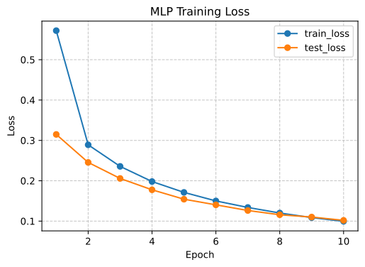
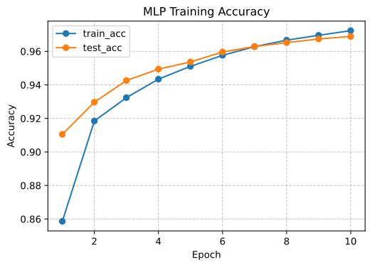
If training is normal, the loss will gradually decrease and the accuracy will gradually increase.
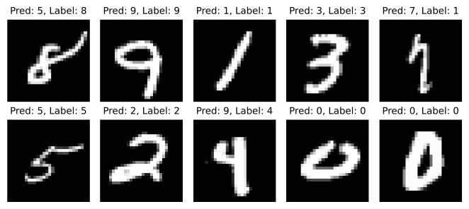
Of course, we can also visualize the model’s predictions:
indices = torch.randperm(len(test_ds))[:10]x_samples = torch.stack([test_ds[i][0] for i in indices])y_samples = torch.tensor([test_ds[i][1] for i in indices])model.cpu().eval()with torch.inference_mode(): logits = model(x_samples) y_preds = logits.argmax(dim=1)fig = plt.figure(3, figsize=(7, 3.2))axes = fig.subplots(2, 5)for i, ax inenumerate(axes.ravel()): ax.imshow(x_samples[i].reshape(28, 28), cmap='gray') ax.axis('off') ax.set_title(f'Pred: {y_preds[i]}, Label: {y_samples[i]}', fontsize=10)fig.tight_layout()plt.show()
3.8.8 Correspondence Between the NumPy Implementation and the PyTorch Implementation
At this point, we have implemented the same MLP in two ways. Their correspondence can be summarized as follows:
Table 3.8.8 Correspondence between the handwritten NumPy version and the PyTorch version
Handwritten NumPy version
PyTorch version
Linear.forward
nn.Linear
ReLU.forward
nn.ReLU
CrossEntropyLoss.forward
nn.CrossEntropyLoss
handwritten backward
loss.backward()
param -= lr * grad
optimizer.step()
handwritten mini-batch indexing
DataLoader
handwritten evaluation loop
model.eval() + torch.no_grad()
So PyTorch does not change the mathematical nature of neural network training. It mainly automates three things for us:
automatically recording the computation graph;
automatically computing gradients;
managing parameters and optimizers through a unified interface.
This is also why the handwritten NumPy version earlier was important: it is the foundation of all neural network training. Once you understand the handwritten version, PyTorch code will no longer make loss.backward() feel like a black box.
3.8.9 Summary
In this section, we reimplemented the two-layer MLP from earlier using PyTorch nn.Module.
In the NumPy version, we needed to implement Linear, ReLU, and CrossEntropyLoss ourselves, and write backward for every layer. In the PyTorch version, these modules are already wrapped as nn.Linear, nn.ReLU, and nn.CrossEntropyLoss, while backpropagation is automatically handled by loss.backward().
However, the mathematical structure behind the two versions is the same: the input passes through linear layers and nonlinear activation functions to produce logits, cross entropy measures the gap between predictions and labels, and parameters are finally updated along the gradient direction.
At this point, we have completed the full training process of an MLP:
Congratulations! You have learned how to build a basic neural network and understand every step of training. In later sections, we will continue to introduce more model components and training techniques on top of this foundation. But no matter how complex a model becomes, it essentially evolves from this basic training process. Once you understand it, you understand the core of deep learning.