4.9 Learning Rate Schedulers: Letting the Learning Rate Change During Training
Author
jshn9515
Published
2026-06-05
Modified
2026-06-05
In the previous sections, we have treated the learning rate \(\eta\) as a hyperparameter in the optimizer. Whether we use SGD, momentum, Adagrad, RMSprop, Adam, or AdamW, the parameter update always contains some form of “step size”:
Different optimizers change how \(\mathrm{update}_t\) is computed. For example, momentum smooths the gradient direction, Adam uses both first-order and second-order moments to adjust the update, and AdamW decouples weight decay from the gradient update.
But there is still one unresolved question:
Does the learning rate have to stay unchanged from the beginning to the end of training?
In many cases, the answer is no.
At the beginning of training, the parameters are usually still far away from a good region. At this stage, we often want a relatively large learning rate so that the model can move quickly toward a lower-loss region. Later in training, the model is already close to a good region. If the learning rate is still large, the parameters may oscillate around the low-loss region and fail to converge further. At this stage, we usually want the learning rate to gradually become smaller so that parameter updates become more refined.
This is the problem that a learning rate scheduler is designed to solve.
A learning rate scheduler does not change the update rule of the optimizer itself. Instead, it controls how the learning rate inside the optimizer changes during training.
The optimizer answers this question:
Given the current learning rate and gradients, how should the parameters be updated?
The learning rate scheduler answers this question:
At this point in training, what should the learning rate be?
In this section, we will not implement schedulers ourselves. Instead, we will summarize common learning rate scheduling strategies from an intuitive perspective, and finally demonstrate their basic usage in PyTorch.
import dnnlpyimport dnnlpy.optim as doptimport matplotlib.pyplot as pltimport numpy as npimport torchimport torch.nn as nnimport torch.optim as optimimport torch.optim.lr_scheduler as lrdnnlpy.set_matplotlib_format('svg')print('PyTorch version:', torch.__version__)
PyTorch version: 2.14.0+cpu
4.9.1 Why Do We Need Learning Rate Scheduling?
If the learning rate is fixed, training may run into two types of problems.
The first problem is that the learning rate is too small. The model updates are stable, but each step is very small, so training may take a long time before reaching a good region.
The second problem is that the learning rate is too large. The model may descend quickly at first, but later it may oscillate around a low-loss region and struggle to converge further. In severe cases, training may even diverge.
So, a natural idea is:
Use a larger learning rate early in training for fast exploration, and use a smaller learning rate later in training for gradual convergence.
This is the basic intuition behind most learning rate schedulers.
For example, when training a CNN, we may first train with lr=0.1 for a while, then reduce the learning rate to 0.01, and then reduce it again to 0.001. This lets the model descend quickly in the early stage and approach a good set of parameters more stably in the later stage.
When training Transformer or ViT models, we often see another strategy: first perform warmup, which gradually increases the learning rate from a very small value, and then slowly decays it. This can avoid the instability caused by using a large learning rate immediately at the beginning of training, when both the parameters and optimizer states are still unstable.
Therefore, a learning rate scheduler is essentially a mechanism for dynamically controlling the optimization step size during training.
4.9.2 The Relationship Between Learning Rate Schedulers and Optimizers
In PyTorch, a scheduler usually wraps an optimizer:
Here, the optimizer is responsible for actually updating the parameters, while the scheduler is responsible for modifying the learning rate inside the optimizer.
In other words, a scheduler does not replace:
optimizer.step()
Instead, it adds one extra step:
scheduler.step()
A common way to use an epoch-level scheduler is:
for epoch inrange(num_epochs): train_one_epoch(model, train_loader, optimizer) scheduler.step()
For a batch-level scheduler such as OneCycleLR, it is usually called after every mini-batch:
for epoch inrange(num_epochs):for x, y in train_loader: optimizer.zero_grad() loss = compute_loss(model, x, y) loss.backward() optimizer.step() scheduler.step()
Therefore, when using a scheduler, one very important question is:
Should this scheduler be called once per epoch, or once per batch?
Different schedulers expect different calling frequencies. If the calling frequency is wrong, the learning rate will change at a completely different speed.
4.9.3 Overview of Common Learning Rate Schedulers
The following table summarizes common learning rate schedulers in PyTorch. Here, we only list the types that are most common and most likely to appear in deep learning training.
Table 1: Comparison of common learning rate schedulers in PyTorch
Scheduler
Core idea
Suitable scenarios
Calling frequency
StepLR
Multiply the learning rate by gamma every fixed number of epochs
Simple baselines and classic CNN training
Usually every epoch
MultiStepLR
Decay the learning rate at specified milestones
Classic vision training recipes, such as reducing LR at several fixed epochs
Usually every epoch
ExponentialLR
Multiply by a fixed factor gamma at every call
When smooth exponential decay is desired
Usually every epoch
CosineAnnealingLR
Smoothly decay from the initial learning rate to a smaller value following a cosine curve
Transformer, ViT, modern vision training, and fine-tuning
Every epoch or every step, depending on the design of T_max
CosineAnnealing WarmRestarts
Periodically restart to a larger learning rate after cosine decay
When periodically re-exploring the parameter space is desired
Usually every epoch or at a finer granularity
ReduceLROnPlateau
Reduce the learning rate when a validation metric stops improving
When metrics fluctuate, the number of training epochs is not fixed, or it is unclear when LR should be reduced
After each validation phase
OneCycleLR
Increase the learning rate first and then decrease it, usually updating every batch
Fast training, super-convergence, and experiments requiring a strong schedule
Every batch
CyclicLR
Cycle the learning rate within a range
When a periodic learning rate change is desired during training
Every batch
LinearLR
Linearly increase or decrease the learning rate
Warmup or simple linear decay
Every epoch or every step
SequentialLR
Chain multiple schedulers stage by stage
Combined strategies such as warmup + cosine decay
Depends on the child schedulers
LambdaLR
Define the learning rate schedule with a custom function
When a fully customized schedule is needed
Depends on the design
At the same time, you can first remember a simple rule of thumb:
For the simplest learning rate schedule: use StepLR or MultiStepLR.
For smooth learning rate decay: use CosineAnnealingLR.
To reduce the learning rate when validation performance plateaus: use ReduceLROnPlateau.
To perform warmup followed by decay: use LinearLR with SequentialLR, or use LambdaLR for custom schedules.
To precisely control the learning rate at every mini-batch: use OneCycleLR.
4.9.4 StepLR and MultiStepLR: Reducing the Learning Rate at Fixed Points
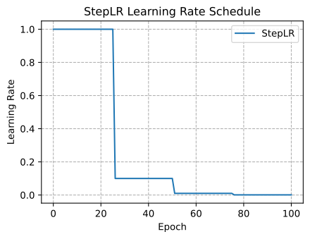
The simplest learning rate scheduling method is step decay. The idea is straightforward: first train with a relatively large learning rate for some time, and after the model has descended to some extent, multiply the learning rate by a factor gamma smaller than 1.
For example, StepLR decays the learning rate every fixed number of epochs:
This means that every 25 epochs, the learning rate becomes 0.1 times its previous value. If the initial learning rate is 1, then the learning rate changes roughly as follows:
1 -> 0.1 -> 0.01 -> 0.001
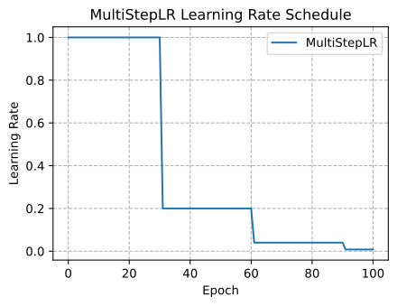
MultiStepLR is a bit more flexible. Instead of decaying at fixed intervals, it decays at specified milestones:
This form is very common in classic vision training. For example, when training a CNN for a fixed number of epochs, we can specify in advance at which epochs the learning rate should be reduced.
Their advantages are simplicity, controllability, and reproducibility. The disadvantage is that we need to know in advance when the learning rate should be reduced. If the training process does not behave as expected, fixed milestones may not be flexible enough.
4.9.5 ExponentialLR: Continuous Exponential Decay
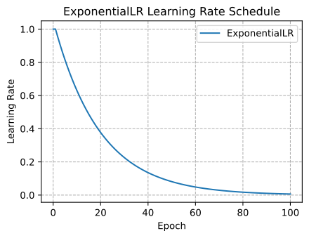
ExponentialLR multiplies the learning rate by the same factor gamma every time it is called:
If it is called once per epoch, then the learning rate changes in the following form:
\[
\eta_t = \eta_0 \cdot \gamma^t
\]
Compared with the sudden drops in StepLR, ExponentialLR changes the learning rate more smoothly. It is suitable when we want the learning rate to continuously decrease but do not want to manually set multiple milestones.
However, it also has a problem: if gamma is too small, the learning rate will decay too early; if gamma is too close to 1, the change may be too slow. So although it is simple, it still requires tuning.
4.9.6 CosineAnnealingLR: Smoothly Decaying to a Smaller Learning Rate
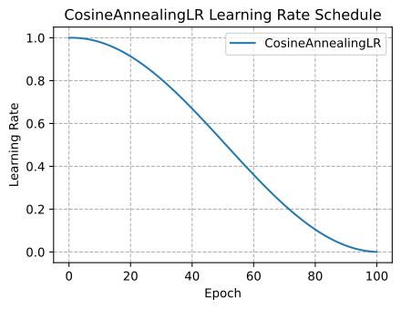
In modern deep learning training, a very common choice is cosine annealing. Its intuition is: instead of suddenly lowering the learning rate, let the learning rate slowly decrease along a smooth curve.
The learning rate will smoothly decrease from the initial value to around eta_min. Compared with StepLR, a cosine schedule does not suddenly cut the learning rate at a particular epoch. Instead, it gradually decreases the learning rate throughout training. This type of schedule is very common in Transformer, ViT, and many modern training recipes. In particular, when the total number of training steps is known, cosine decay is easy to use: simply set T_max to the total number of epochs or total number of steps.
One thing to note is that the unit of T_max depends on how you call scheduler.step().
So the parameters of a scheduler cannot be understood separately from its calling frequency.
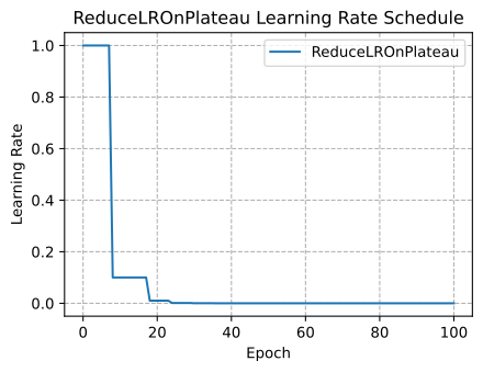
4.9.7 ReduceLROnPlateau: Reducing the Learning Rate When a Metric Stagnates
The StepLR, MultiStepLR, ExponentialLR, and CosineAnnealingLR schedulers above are all pre-arranged schedules. They do not care about validation metrics; they only change the learning rate according to epochs or steps. But sometimes we do not know when the learning rate should be reduced. For example, the validation loss may stagnate at some stage, but we cannot know in advance at which epoch this will happen.
This is a little different from ordinary schedulers. Ordinary schedulers usually do not need a metric:
scheduler.step()
But ReduceLROnPlateau needs to know the current monitored metric:
scheduler.step(metric)
It is suitable for tasks where the training process is uncertain and validation metrics are important. Its downside is that it depends on validation metrics, so if the validation metric is noisy, the learning rate changes may also be affected.
4.9.8 Warmup: Slowly Increasing the Learning Rate at the Beginning of Training
So far, we have been talking about how the learning rate gradually becomes smaller. But in many modern models, training starts by increasing the learning rate from a very small value to a larger value, and then gradually decreasing it. This strategy is called warmup.
The intuition behind warmup is:
At the beginning of training, the parameters, gradient distribution, and optimizer states are all still unstable, so do not use the maximum learning rate immediately.
This is especially relevant for adaptive optimizers such as AdamW. In the first few training steps, both the first-moment and second-moment estimates are still unstable. Warmup is also commonly used in Transformer training, where the learning rate is first increased linearly and then enters a decay phase.
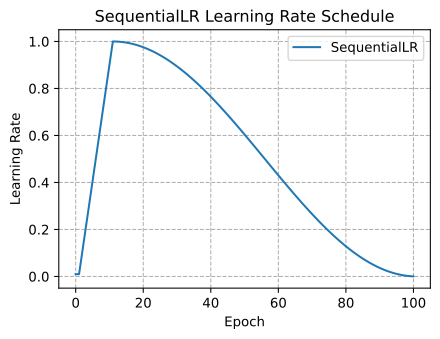
In PyTorch, we can implement warmup + cosine decay using LinearLR together with SequentialLR:
This means: use linear warmup for the first warmup_steps steps, and then switch to cosine decay.
This combination is very common in modern training. First, warm up to avoid instability at the beginning of training; then decay so that training can converge more stably in the later stage.
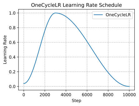
4.9.9 OneCycleLR: A Strong Schedule That Increases First and Then Decreases
OneCycleLR (Smith and Topin 2018) uses the 1cycle policy. Its characteristic is that the learning rate first increases from a smaller value to a larger value, and then gradually decreases to a very small value. The PyTorch documentation also notes that OneCycleLR is usually called once per batch, not once per epoch.
for epoch inrange(num_epochs):for x, y in train_loader: optimizer.zero_grad() loss = compute_loss(model, x, y) loss.backward() optimizer.step() scheduler.step()
It is suitable when we want to train quickly using a relatively large learning rate. Compared with simple decay, OneCycleLR has stronger control over the training process, but it also depends more on max_lr, the total number of steps, and batch-level calling. So if we only want to write a relatively stable baseline, AdamW + cosine decay is usually simpler; if we want to try fast training or super-convergence, OneCycleLR is worth considering.
4.9.10 LambdaLR: Defining a Custom Schedule with a Function
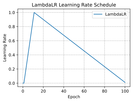
Sometimes, PyTorch’s built-in schedulers cannot fully express the learning rate curve we want. In that case, we can use LambdaLR. LambdaLR takes a function and multiplies the initial learning rate by the scaling factor returned by that function.
For example, the following implements a simple linear warmup + linear decay schedule:
This style is very flexible and is suitable for reproducing custom schedules from papers or frameworks. The downside is that the function is defined by us, so it is easier to make mistakes. For teaching and ordinary training, we can prioritize schedulers that PyTorch has already packaged.
4.9.11 PyTorch Demo: How to Use a Scheduler in a Training Loop
Finally, let us look at a style that is closer to real training.
For most epoch-level schedulers, such as StepLR, ExponentialLR, and CosineAnnealingLR, the common pattern is:
num_epochs =100model = nn.Linear(1, 1)optimizer = torch.optim.AdamW( model.parameters(), lr=1e-3, weight_decay=1e-2,)scheduler = lr.CosineAnnealingLR( optimizer, T_max=num_epochs,)for epoch inrange(num_epochs): model.train()for x, y in train_loader: optimizer.zero_grad() pred = model(x) loss = compute_loss(pred, y) loss.backward() optimizer.step() scheduler.step()
For ReduceLROnPlateau, the call is usually placed after validation, and a validation metric needs to be passed in:
Note that the scheduler parameters must be consistent with how often scheduler.step() is called. If T_max is the number of epochs, call it once per epoch; if T_max is the total number of steps, call it once per mini-batch.
After understanding these basic usages, when we see various optimizer + scheduler combinations in real training, their design intent and usage will become much clearer.
4.9.12 Summary
In this section, we introduced learning rate schedulers. The optimizer decides “given the gradients and learning rate, how should the parameters be updated,” while the scheduler decides “at the current stage of training, what should the learning rate be.”
A fixed learning rate is simple, but the same step size is not necessarily suitable for the entire training process. In the early stage of training, a larger learning rate is usually needed for fast descent; in the later stage, a smaller learning rate is usually needed for stable convergence. In Transformer, ViT, and large model training, warmup is also commonly used to reduce instability at the beginning of training.
Common schedulers can be divided into several types:
StepLR and MultiStepLR perform stepwise decay;
ExponentialLR performs exponential decay;
CosineAnnealingLR performs smooth cosine decay;
ReduceLROnPlateau automatically lowers the learning rate when a validation metric stagnates;
OneCycleLR uses a strong schedule that increases first and then decreases;
LinearLR, SequentialLR, and LambdaLR are often used for warmup or custom schedules.
In practice, we can first remember a few default choices: if the total number of training steps is known, AdamW + warmup + cosine decay is a very common starting point for modern models; if we are training a classic CNN, SGD + momentum with StepLR or MultiStepLR is still very common; if the validation metric clearly stagnates, we can consider ReduceLROnPlateau; if we want to try fast training, we can consider OneCycleLR.
At this point, we have completed the main thread of this chapter: from the most basic SGD and momentum, to adaptive learning rates, Adam, AdamW, Muon, optimizer selection, and learning rate scheduling. After understanding these ideas, many seemingly complex optimizer and scheduler combinations in later CNN, Transformer, ViT, or large model training configurations will become much easier to understand.
References
Smith, Leslie N., and Nicholay Topin. 2018. Super-Convergence: Very Fast Training of Neural Networks Using Large Learning Rates. https://arxiv.org/abs/1708.07120.