In the previous chapters, we have seen that a neural network can be viewed as a function with parameters. Given an input \(x\), the model produces a prediction through forward propagation, and then a loss function measures the gap between the prediction and the true label. The goal of training is to keep adjusting the model parameters so that the loss becomes smaller and smaller.
If we use \(\theta\) to denote all learnable parameters in the model, and \(L(\theta)\) to denote the loss under the current parameters, then training a neural network is essentially solving an optimization problem:
\[
\min_\theta L(\theta)
\]
This sentence looks simple, but behind it lies a very important question:
How do we know in which direction the parameters should be updated?
Automatic differentiation can help us compute gradients. For a parameter \(\theta\), the gradient \(\nabla_\theta L(\theta)\) tells us how the loss would change if we slightly changed the parameter. However, knowing the gradient is not the same as knowing the full training procedure. The gradient only tells us a local direction. When actually training a model, we still need to decide:
which direction the parameters should move in;
how far they should move each time;
how much data should be used to estimate this direction.
In this section, we start from the most basic form of gradient descent and clarify the basic logic of “updating parameters according to gradients.” Then we will discuss why, in deep learning, the more common method is not full gradient descent, but stochastic gradient descent, usually called SGD (Stochastic Gradient Descent)(Bottou 2012).
from collections.abc import Iterablefrom typing import overrideimport dnnlpyimport dnnlpy.optim as doptimport matplotlib.pyplot as pltimport torchimport torch.nn as nnimport torch.nn.functional as Fimport torch.optim as optimfrom torch import Tensordnnlpy.set_matplotlib_format('svg')print('PyTorch version:', torch.__version__)
PyTorch version: 2.14.0+cpu
4.1.1 What Does the Gradient Tell Us?
First, consider the simplest case: there is only one parameter \(\theta\), and the loss function is \(L(\theta)\).
If we stand at the current parameter position \(\theta_t\), the gradient
\[
\frac{dL}{d\theta}
\]
represents the direction in which the loss function changes at this position.
If the gradient is positive, it means that when \(\theta\) increases, the loss also increases. To make the loss smaller, we should move \(\theta\) in the smaller direction. If the gradient is negative, it means that when \(\theta\) increases, the loss decreases. To make the loss smaller, we should move \(\theta\) in the larger direction.
So regardless of whether the gradient is positive or negative, if we want the loss to decrease, a natural choice is to update the parameter in the opposite direction of the gradient:
Intuitively, gradient descent is like walking downhill on a slope. The gradient at the current position tells us the steepest uphill direction, while the negative gradient direction is the steepest downhill direction. Each time, we take a small step along the negative gradient direction, hoping to gradually reach a position with lower loss.
Of course, choosing the learning rate \(\eta\) is also very important. If the learning rate is too small, each step is very cautious, and training becomes slow. The loss may decrease steadily, but it may take many iterations to approach good parameters. If the learning rate is too large, each step may go too far, or even jump directly over the minimum. In more severe cases, the parameters may oscillate back and forth on the loss surface, the loss may increase instead of decrease, and training becomes unstable. Therefore, the learning rate is one of the most important hyperparameters in optimization.
We can think of the learning rate as the model’s degree of trust in the gradient. A larger learning rate means the model is more aggressive and believes it can move far along the current gradient direction. A smaller learning rate means the model is more conservative and only moves a little bit along the current direction.
In later chapters, we will see that the core ideas of many optimizers are actually related to the learning rate. For example, Adagrad, RMSprop, and Adam automatically adjust the learning rate for different parameters; learning rate schedulers change the global learning rate during training. But in the most basic gradient descent, the learning rate is just a fixed manually set number.
4.1.2 Observing Gradient Descent with a Simple Example
To understand gradient descent more intuitively, let us ignore neural networks for now and look at a simple function:
\[
L(\theta) = 0.1 (x - 2)^2 + 2.0 (y + 1)^2
\]
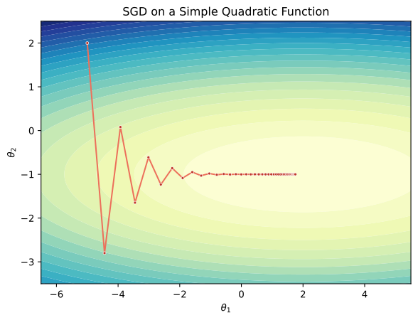
The minimum of this function clearly appears at \((x, y) = (2, -1)\). If we start from a faraway position, such as \((x, y) = (-5, 2)\), gradient descent should push the parameters step by step toward \((2, -1)\).
Final theta: tensor([ 1.7508, -1.0000])
Final loss: 0.0062118638306856155
We can plot the parameter update trajectory:
x = torch.linspace(-6.5, 5.5, 200)y = torch.linspace(-3.5, 2.5, 200)X, Y = torch.meshgrid(x, y, indexing='ij')Z =0.1* (X -2) **2+2.0* (Y +1) **2fig = plt.figure(1)ax = fig.add_subplot(1, 1, 1)ax.contourf(X, Y, Z, levels=25, cmap='YlGnBu')ax.plot( history[:, 0], history[:, 1], color='#EC705B', marker='o', markersize=3, markerfacecolor='#C0392B', markeredgecolor='white', markeredgewidth=0.5,)ax.set_xlabel(r'$\theta_1$')ax.set_ylabel(r'$\theta_2$')ax.set_title('SGD on a Simple Quadratic Function')plt.show()
From the figure, we can see that the parameters are far from the optimum at the beginning, and the gradient is large, so each step is also relatively obvious. As the parameters gradually approach \((2, -1)\), the gradient becomes smaller and smaller, and the update step size naturally becomes smaller as well. This reflects a basic property of gradient descent: even if the learning rate is fixed, the actual update amount is still affected by the gradient magnitude. When far from the minimum, the gradient is usually large, so the parameters move quickly; when close to the minimum, the gradient becomes smaller, so the parameters move more slowly.
4.1.3 From a Single Sample to the Entire Dataset
In the example above, the loss function was only a simple formula. But in real supervised learning tasks, we usually have a training set:
If we want to update parameters strictly according to gradient descent, we need to compute the average loss over the entire training set and then take its gradient:
This is usually called batch gradient descent, meaning that every update uses the entire training set.
This approach is mathematically clean. Each time, we are indeed using the gradient of the full training objective, so the direction is relatively stable and is not affected by the noise of individual samples. But the problem is also obvious: when the training set is large, every parameter update requires going through all data, which is too expensive.
Imagine that we have millions of images. If each single parameter update requires running forward propagation and backward propagation on all images, training will be extremely slow. More importantly, in deep learning, we usually need to update parameters for thousands or even tens of thousands of steps. If every step uses the full training set, the computational cost becomes enormous.
Therefore, although batch gradient descent is conceptually simple, it is not the most commonly used form in modern deep learning training.
4.1.4 Stochastic Gradient Descent: We Do Not Need to Look at the Full Dataset Every Time
Since using the full training set every time is too expensive, a natural question is:
Can we look at only part of the data each time and still roughly know where the parameters should go?
This is the core idea of stochastic gradient descent.
The most extreme approach is to randomly sample only one example \((x_i, y_i)\) each time and use the gradient of this sample’s loss to approximate the gradient of the full training set:
This is stochastic gradient descent in its original sense.
Its advantage is that each update is very cheap, because it only needs to compute the gradient of one sample. The disadvantage is that the direction can be quite noisy. A single sample may not represent the entire training set, so each step’s direction may be biased, and sometimes it may even temporarily increase the overall loss. But in the long run, if the samples are randomly drawn, these noisy update directions will fluctuate around the true gradient direction. The model no longer moves in the direction that decreases the overall loss most precisely at every step; instead, it gradually approaches a good region through noise.
This noise is not entirely bad. On the non-convex loss surfaces of deep learning, a suitable amount of randomness can sometimes help the model escape certain narrow or poor regions. However, too much noise can also make training unstable. Therefore, in practice, we rarely use only one sample each time. Instead, we use mini-batches.
4.1.5 Mini-batch SGD: The Default Training Method in Deep Learning
In modern deep learning, when we say SGD, we often mean mini-batch SGD. That is, each time we use neither one sample nor the entire training set, but instead randomly sample a small batch of examples:
\[
\mathcal{B} = \{(x_i, y_i)\}_{i \in B}
\]
Then we compute the average loss on this mini-batch:
Mini-batch SGD lies between full batch gradient descent and single-sample SGD. If the batch size is large, the gradient estimate is more stable, but each step costs more computation and the number of updates becomes smaller. If the batch size is small, each step is cheaper and updates happen more frequently, but the gradient noise is larger and training may become more jittery. Therefore, mini-batch training is essentially a trade-off between computational efficiency and the quality of gradient estimation.
From an implementation perspective, the common training loop in PyTorch is actually the form of mini-batch SGD:
model = nn.Linear(1, 1)optimizer = optim.SGD(model.parameters(), lr=0.1)x = torch.randn(32, 1)y =2* x +1pred = model(x)loss = F.mse_loss(pred, y)optimizer.zero_grad()loss.backward()optimizer.step()print('Mini-batch loss:', loss.item())
Mini-batch loss: 1.006398320198059
Here, x and y are one mini-batch. loss.backward() computes the gradients on the current mini-batch and stores them in the .grad attributes of the model parameters, while optimizer.step() updates the parameters according to these gradients.
If we use mini-batches each time, there is another question: how should these mini-batches be selected?
The usual practice is to shuffle the training data at the beginning of each epoch and then split it into mini-batches in order. This prevents the model from always seeing the data in a fixed order.
If the data is not shuffled, there may be strong bias between mini-batches. For example, in a classification dataset, the first part may contain only cats and the later part only dogs. If we do not shuffle the data, the model sees only cats in the first few steps and only dogs in the later steps, making the gradient direction very unstable. The purpose of shuffling is to make each mini-batch as close as possible to a small random sample of the full training set. In this way, although the mini-batch gradient still contains noise, it at least will not be biased toward one class for a long time.
This is also why, in PyTorch’s DataLoader, the training set is usually configured with shuffle=True.
Validation and test sets usually do not need shuffle=True. During validation and testing, parameters are not updated. We only need to evaluate model performance stably, and the data order does not affect the final average metric.
4.1.7 Weight Decay in SGD
The SGD we discussed earlier only cares about one thing: reducing the training loss. In other words, the parameter update is entirely determined by the gradient on the current mini-batch:
\[
\theta_{t+1} = \theta_t - \eta g_t
\]
where \(g_t = \nabla_\theta L_{\mathcal{B}}(\theta_t)\). However, when training neural networks, we usually hope the model not only performs well on the training set, but also generalizes well to unseen data. To improve generalization, we often use regularization methods to constrain model complexity.
A common approach is to add an extra penalty term to the loss function, encouraging the model to use smaller weights:
Here, \(\lambda\) is the regularization strength, controlling how strongly we want the parameters to become smaller. \(||\theta||_2^2\) denotes the sum of squared parameters. The larger this term is, the larger the parameters are overall. After adding this term, the optimizer must not only reduce the original training loss, but also avoid making the parameters grow without bound.
This is usually called L2 regularization. In SGD, it is also often called weight decay.
The name comes from its effect on the parameter update. Since:
This step is important. In addition to the normal gradient update \(-\eta g_t\), the parameter itself is multiplied by a coefficient smaller than 1, \((1 - \eta\lambda)\). In other words, each update slightly decays the weights toward 0, which is why it is called weight decay.
Intuitively, ordinary SGD only asks:
How should the parameters move to reduce the loss of the current batch?
SGD with weight decay asks one more question:
While reducing the loss, can we also keep the parameters from becoming too large?
So weight decay can be viewed as a way to constrain model complexity. It does not directly reduce the number of model parameters; instead, it encourages the model to use smaller weights.
In basic SGD, implementing weight decay is very simple. We only need to add \(\lambda \theta\) to the gradient before updating the parameter:
class SimpleSGDWithWeightDecay(dopt.Optimizer):def__init__(self, params: Iterable[Tensor], lr: float=1e-3, weight_decay: float=0.0, ):super().__init__(params)self.lr = lrself.weight_decay = weight_decay@override@torch.no_grad()def step(self):for p inself.params:if p.grad isNone:continue grad = p.gradifself.weight_decay >0: grad = grad.add(p, alpha=self.weight_decay) p.sub_(grad, alpha=self.lr)
Note that weight_decay here does not subtract a fixed value directly from the parameters. Instead, it decays the parameters proportionally according to their current magnitude. The larger the parameter is, the larger the decay term; the closer the parameter is to 0, the smaller the decay term.
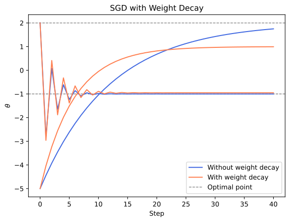
We can use the same simple quadratic function to see its effect:
Without weight decay:
Final theta: tensor([ 1.7508, -1.0000])
Final loss: 0.0062118638306856155
With weight decay:
Final theta: tensor([ 0.9944, -0.9524])
Final loss: 0.10566135495901108
Without weight decay, the parameters gradually approach the optimum of the original loss function, \((2, -1)\). After adding weight decay, the parameters are affected by an extra force pulling them back toward 0, so in the end \(x\) stops at a position smaller than 2, and \(y\) stops at a position greater than -1. This does not mean the optimizer is wrong. It is because the optimization objective has changed. After adding weight decay, the optimizer is no longer only minimizing
Therefore, the new optimum lies between the original optimum and 0.
In PyTorch, optim.SGD also provides a weight_decay argument:
model = nn.Linear(1, 1)optimizer = optim.SGD( model.parameters(), lr=0.1, weight_decay=1e-4,)
However, it is worth noting that we usually do not apply weight decay to all parameters. For example, the bias in Linear layers, and the scale and shift parameters in LayerNorm, are often not decayed, because these parameters are not ordinary weights of linear or convolutional layers, and decaying them is not necessarily helpful. In real projects, different weight_decay values are often assigned to different parameters through parameter groups. We mentioned this earlier in the chapter on PyTorch optimizers.
4.1.8 Advantages and Problems of SGD
At this point, we can summarize why SGD is important.
First, SGD makes large-scale training feasible. The model does not need to go through the full training set for every update. Instead, it can use mini-batch gradients to approximate the full gradient, greatly reducing the cost of each update.
Second, the update rule of SGD is very simple:
\[
\theta_{t+1} = \theta_t - \eta g_t
\]
where \(g_t\) is the gradient on the current mini-batch. Precisely because it is simple, we can more clearly see what later optimizers improve. Momentum modifies the update direction and gives parameter updates inertia; Adagrad, RMSprop, and Adam modify the effective learning rate of different parameters; AdamW re-handles the relationship between weight decay and gradient updates.
However, SGD itself also has obvious problems.
The first problem is that the update direction can be jittery. The mini-batch gradient is only an estimate of the full gradient, and different batches may vary greatly, so the parameter update trajectory can be noisy.
The second problem is that all parameters share the same learning rate. Whether one parameter often has large gradients or another parameter has very small gradients for a long time, basic SGD uses the same \(\eta\) to control their updates. This may not be flexible enough in complex neural networks.
The third problem is that SGD does not remember past gradients. Each update only looks at the gradient of the current mini-batch, and past update directions do not directly affect the current update. This can cause parameters to oscillate back and forth in some directions, especially when the loss surface is long and narrow.
These are exactly the problems that later optimizers try to solve.
Momentum asks: since the current gradient contains noise, can we refer to the update direction over a recent period of time?
Adagrad and RMSprop ask: since different parameters have different gradient scales, can we assign a different learning rate to each parameter?
Adam asks: can we combine momentum’s direction smoothing with RMSprop’s adaptive scaling?
Therefore, SGD is not only a basic optimizer; it is also the starting point for understanding all later optimizers.
4.1.9 Summary
In this section, we started from the most basic question: after we have gradients, how should the parameters be updated?
The gradient tells us the direction in which the loss increases fastest, so the negative gradient direction is the local direction of fastest descent. The core idea of gradient descent is to update parameters along the negative gradient direction and use the learning rate to control how far each step goes.
For the full training set, batch gradient descent uses all samples to compute the gradient each time. Its direction is stable, but the computational cost is high. Stochastic gradient descent uses the gradient of random samples or mini-batches to approximate the full gradient, greatly reducing the cost of each update while also introducing a suitable amount of randomness.
In modern deep learning, we usually use mini-batch SGD. It strikes a balance between computational efficiency and gradient stability, and it is the basic form of neural network training. The common PyTorch training workflow with zero_grad(), backward(), and step() is essentially computing gradients and updating parameters on mini-batches.
In addition, we introduced weight decay in SGD. It can be understood as adding an L2 regularization term to the loss function, encouraging parameters to remain small while reducing the training loss. For basic SGD, L2 regularization and weight decay are equivalent. But for adaptive optimizers such as Adam, the two lead to different behavior, so we will return to this issue later when discussing AdamW.
However, basic SGD also has limitations: its update direction is easily affected by mini-batch noise, all parameters share the same learning rate, and it does not remember past gradient directions. In the next section, we will see that momentum is the first important improvement to SGD that starts from these problems.