In the previous section, we went from gradient descent to mini-batch SGD. The update rule of SGD is very simple:
\[
\theta_{t+1} = \theta_t - \eta g_t
\]
Here, \(g_t\) is the gradient on the current mini-batch.
The intuition behind this formula is clear: the current gradient points in the direction where the loss increases the fastest, so we take one step in the negative gradient direction. However, SGD has an obvious problem:
Each step only trusts the gradient of the current mini-batch.
If the gradient direction of the current mini-batch is accurate, the update will be smooth. If the current mini-batch contains noise, the update direction will fluctuate. The loss surface in deep learning is usually complex: some directions are steep, while others are flat. SGD may oscillate back and forth along steep directions, while moving very slowly along flat directions.
The Momentum method (Sutskever et al. 2013) that we will discuss in this section is a very natural idea proposed to address this problem:
Do not only look at the gradient of the current step; also refer to the update directions from the recent past.
from collections.abc import Iterablefrom pprint import pprintfrom typing import overrideimport dnnlpyimport dnnlpy.optim as doptimport matplotlib.pyplot as pltimport torchimport torch.nn as nnimport torch.nn.functional as Fimport torch.optim as optimfrom torch import Tensordnnlpy.set_matplotlib_format('svg')print('PyTorch version:', torch.__version__)
PyTorch version: 2.14.0+cpu
4.2.1 Why Does SGD Oscillate?
To understand momentum, let us first look at when SGD performs poorly.
Consider a two-dimensional parameter:
\[
\theta = (x, y)
\]
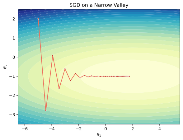
Suppose the loss function is shaped like a long, narrow valley. Along the \(x\) direction, the loss changes quickly; along the \(y\) direction, the loss changes slowly. Such loss surfaces are not uncommon in neural network training.
If we use SGD to update the parameters, the negative gradient direction may not always move exactly along the bottom of the valley. Because some directions are very steep, the gradient may mainly point toward the sides of the valley, causing the parameters to oscillate between the two sides. Meanwhile, the direction in which we should actually move forward progresses very slowly. This is like a person walking downhill in a long, narrow valley: each step is determined only by the slope under their feet. Because the sides are very steep, the person may keep bumping into the left side and then the right side. Although they are generally descending, the path is very winding.
We can simulate this situation with a simple quadratic function:
\[
L(\theta) = 0.1(x - 2)^2 + 2.0(y + 1)^2
\]
Here, the \(y\) direction is steeper, while the \(x\) direction is flatter. The minimum is at \((-2, 1)\).
From the figure, we can see that the parameters do not move smoothly toward the lowest point. Instead, they swing back and forth on the steep slopes on both sides. This oscillation wastes many update steps. In fact, if you change the learning rate to 0.5, it may not converge at all.
This leads to a question: if the gradients over many steps roughly point in the same direction, can we make the parameters move faster in that direction? If the gradient in one direction repeatedly flips back and forth, can we cancel out this oscillation?
Momentum does exactly this.
4.2.2 Momentum: Giving the Update Direction Inertia
The core idea of momentum is simple:
The current update direction is not determined only by the current gradient, but also by past update directions.
In ordinary SGD, the update direction at each step is \(-g_t\). Momentum additionally maintains a variable \(v_t\), which can be understood as the “velocity” or “momentum” of the parameter update. At each step, we first update this momentum:
\[
v_t = \beta v_{t-1} + g_t
\]
Then we use this momentum to update the parameters:
\[
\theta_{t+1} = \theta_t - \eta v_t
\]
Here, \(\beta\) is usually called the momentum coefficient, and a common value is 0.9.
The intuition behind this formula is:
\(g_t\) is the current gradient;
\(v_{t-1}\) is the accumulated direction of past gradients;
\(\beta\) controls how much of the past direction is retained.
If the gradients over many consecutive steps point in similar directions, these gradients will keep accumulating, \(v_t\) will become larger, and the parameters will move faster in that direction. If the gradient in one direction is positive at one moment and negative at another, these gradients will cancel each other out. As a result, \(v_t\) will not accumulate much in that direction, and the oscillation will be weakened.
Therefore, momentum does two things at the same time:
It accelerates along consistent directions;
It smooths directions that repeatedly oscillate.
This is why momentum is often explained as “inertia.” Ordinary SGD decides the direction from scratch at every step, while momentum is like a small ball with velocity. It does not immediately make a sharp turn just because the current gradient changes slightly; instead, it preserves the motion trend from the past.
4.2.3 Viewing Momentum as an Exponentially Weighted Average
The formula above is:
\[
v_t = \beta v_{t-1} + g_t
\]
If we expand it, we can see that \(v_t\) contains gradients from many past steps:
In other words, momentum does not only look at the current gradient. It looks at a weighted sum of past gradients. More recent gradients have larger weights, while older gradients have smaller weights.
This matches our intuition during training:
The gradient of the current mini-batch is important;
The gradients from the most recent few steps are also useful references;
Gradients from a long time ago should gradually fade out.
So momentum can be understood as a kind of smoothing over gradient directions. It turns a noisy single-step gradient into a more stable accumulated direction. In this way, inside a long and narrow valley, the parameters will not oscillate back and forth as much, but will move more smoothly along the bottom of the valley.
In fact, if we assume that the gradient direction remains roughly the same for a period of time, and the gradient at every step is the same vector \(g\), the expression above becomes a geometric series:
This shows that when the gradient direction stays consistent across many consecutive steps, momentum makes the update speed roughly \(\frac{1}{1 - \beta}\) times that of ordinary SGD. For example, when \(\beta=0.9\), this acceleration factor is 10. Therefore, when using momentum, the learning rate usually needs to be smaller.
In addition, some textbooks write momentum in another form:
This is slightly different from the previous form. In the first form, \(v_t\) accumulates gradients, and the learning rate \(\eta\) is multiplied only at the final parameter update. In the second form, the gradient is first multiplied by the learning rate and then accumulated into \(v_t\), so \(v_t\) itself represents the step size of a parameter update. If the learning rate \(\eta\) remains unchanged during training and the initial \(v_0 = 0\), these two forms are essentially equivalent up to a constant scaling, and they produce equivalent parameter updates. PyTorch uses the first form.
Regardless of the exact notation, the core idea is:
Momentum accumulates past gradient directions and uses a smoother, more inertial direction to update the parameters.
4.2.4 Comparing the Trajectories of Momentum and SGD
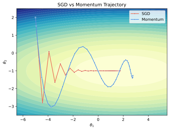
We can implement momentum on the long, narrow valley example above and observe how it differs from ordinary SGD.
First, implement a simple SimpleSGDWithMomentum optimizer:
class SimpleSGDWithMomentum(dopt.Optimizer):def__init__(self, params: Iterable[Tensor], lr: float=1e-3, momentum: float=0.0, ):super().__init__(params)self.lr = lrself.momentum = momentumself.velocity = [torch.zeros_like(p) for p inself.params]@override@torch.no_grad()def step(self):for p, v inzip(self.params, self.velocity, strict=True):if p.grad isNone:continue v.mul_(self.momentum).add_(p.grad) p.sub_(v, alpha=self.lr)
Then compare the trajectories of ordinary SGD and momentum:
Note
Note that when momentum is used, the learning rate usually needs to be smaller. For example, with momentum=0.9, the learning rate often needs to be one order of magnitude smaller than ordinary SGD. Therefore, here we set the learning rate of SGD + momentum to 0.04, while the learning rate of ordinary SGD is set to 0.4.
The trajectory of momentum is usually more continuous. It is not completely determined by the current gradient like ordinary SGD; instead, it continues moving with the direction accumulated from the past. Of course, this does not mean that momentum is always more stable. If the learning rate is too large, or if \(\beta\) is too close to 1, the inertia may become too strong, causing the parameters to overshoot the minimum and produce larger oscillations. Therefore, momentum does not eliminate the need to tune the learning rate; it changes the way the gradient update direction is formed.
4.2.5 Momentum in PyTorch
In PyTorch, optim.SGD already supports momentum. We only need to set the momentum argument:
model = nn.Linear(6, 1)optimizer = optim.SGD( model.parameters(), lr=0.1, momentum=0.9,)
This optimizer is still called SGD, but it is no longer the most naive form of SGD. It maintains a momentum buffer for each parameter, which is the momentum variable we discussed above.
That is, the optimizer internally performs the momentum update inside optimizer.step(). From the user’s perspective, the interface is still: clear gradients, run backpropagation, and update parameters.
If we want to inspect the state maintained by the optimizer, we can look at state_dict(). After step() is called once, PyTorch creates a corresponding momentum buffer for the parameter:
state = optimizer.state_dict()['state']pprint(state)
This also shows an important difference between momentum and ordinary SGD:
A momentum optimizer has state.
Ordinary SGD only needs the current parameters and the current gradients, while momentum also needs to remember the accumulated velocity from the past. Therefore, when saving a model checkpoint, we should not only save the model parameters, but also save the optimizer state. Otherwise, after resuming training, the momentum buffer will be lost, and the training trajectory will change.
4.2.6 Nesterov Momentum: Looking One Step Ahead
The idea of momentum is to let the parameters move forward with inertia. But this also creates a problem: if the inertia is too strong, the parameters may overshoot. Only after the parameters have actually overshot do we realize that the loss surface ahead has become steeper and start slowing down. By then, a few steps may already have been wasted. Is there a way to sense the changes ahead earlier and adjust the velocity accordingly?
Since we are very likely to move along the inertia direction, why not estimate the gradient at the “one-step-ahead” position first?
In other words, ordinary momentum asks: I am standing at \(\theta_t\) right now, what is the gradient here? Nesterov momentum asks: according to the current inertia, I am about to move to some position ahead. What is the gradient at that forward position?
In this way, Nesterov momentum can sense changes ahead earlier. If the loss surface ahead starts becoming steeper, or if the direction needs to be adjusted, it can correct the velocity in advance instead of reacting only after the parameters have already rushed past.
Here, \(\tilde{\theta}_t\) is a lookahead position. We first estimate the position that the parameters may reach next according to the previous momentum direction; then we compute the gradient \(g_t\) at that position and use it to update the momentum and the parameters.
However, note that Nesterov momentum in deep learning frameworks usually does not actually move the parameters to \(\tilde{\theta}_t\) first and then perform another forward and backward pass. This is because in PyTorch’s training workflow, the gradients are computed when loss.backward() is called, while optimizer.step() happens after backpropagation. In other words, when the optimizer starts updating the parameters, p.grad already exists, and it is usually the gradient computed at the current parameters \(\theta_t\).
Therefore, PyTorch uses a Nesterov form that is more suitable for framework implementation. It first updates the momentum just like ordinary momentum:
\[
v_t = \beta v_{t-1} + g_t
\]
Then, instead of directly using \(v_t\) to update the parameters, it uses the following corrected direction:
\[
\beta v_t + g_t
\]
This is equivalent to adding an extra correction term \(\beta v_t\) on top of the current gradient. This correction term can be viewed as an early correction for the next-step inertia direction. Since \(v_t\) is the momentum accumulated up to the current step, \(\beta v_t\) can be understood as the inertia direction that will be used for the next update.
PyTorch-style Nesterov momentum can be written as:
v.mul_(self.momentum).add_(p.grad)p.sub_(self.lr * (self.momentum * v + p.grad))
Therefore, the explicit lookahead version emphasizes moving to \(\tilde{\theta}_t\) first and then computing the gradient there. The PyTorch-style implementation constructs a Nesterov-corrected update direction based on the already available gradient. It is more suitable for the standard training workflow.
Enabling Nesterov momentum in PyTorch is also simple:
Note that PyTorch requires momentum to be positive and dampening to be 0 when using Nesterov momentum. For beginners, there is no need to get stuck on these implementation details at first. Just remember that nesterov=True means using a Nesterov-style momentum correction.
4.2.7 The Role and Limitations of Momentum
Momentum is an important improvement over SGD. It does not change the basic idea of descending along the gradient, but it changes the direction used at each step: instead of only looking at the current gradient, it also takes past gradient directions into account.
Its main effects can be summarized as follows:
Reducing oscillation: if the gradient in one direction keeps changing back and forth, momentum allows the positive and negative directions to cancel each other out, thereby weakening the oscillation.
Accelerating consistent directions: if the gradients over many steps point in similar directions, momentum keeps accumulating that direction, making parameter updates faster.
Introducing optimizer state: because momentum needs to maintain a velocity variable, the optimizer is no longer a stateless update rule.
However, momentum still has an important limitation:
All parameters still share the same global learning rate.
That is, momentum can smooth and accumulate directions, but it does not automatically determine that one parameter should use a larger learning rate while another should use a smaller one. In complex models, however, different parameters may have very different gradient scales. Some parameters frequently receive large gradients, while others have small gradients for a long time. If all parameters use the same learning rate, training may still be insufficiently flexible.
This leads to the next class of optimizers: adaptive learning rate methods. Optimizers starting from Adagrad ask: since different parameters have different gradient histories, can we adjust the learning rate separately for each parameter?
This is exactly the question we will discuss in the next section.
4.2.8 Summary
In this section, we started from the limitations of SGD and introduced momentum.
Ordinary SGD only uses the gradient of the current mini-batch at each step, so its update direction is easily affected by noise. In a long and narrow loss surface, SGD may oscillate back and forth along steep directions while moving slowly in the direction where it should actually progress.
The core idea of momentum is to give parameter updates inertia. It maintains a velocity variable and accumulates past gradient directions. In directions where the gradient stays consistent, the parameters accelerate. In directions where the gradient repeatedly changes, the oscillation is partially canceled out.
Nesterov momentum further proposes that since the parameters will move forward along the inertia direction, we might as well compute the gradient at the position ahead first, so that changes in direction can be sensed earlier. It can be viewed as a “lookahead” correction to ordinary momentum.
However, momentum and Nesterov momentum still use a global learning rate. They solve the problem of noisy update directions and lack of inertia, but they do not solve the problem of whether different parameters should have different learning rates. In the next section, we will see that Adagrad starts exactly from this question and introduces an adaptive learning rate for each parameter.
References
Sutskever, Ilya, James Martens, George Dahl, and Geoffrey Hinton. 2013. On the Importance of Initialization and Momentum in Deep Learning. (Atlanta, Georgia, USA), Proceedings of machine learning research, vol. 28 (3): 1139–47. https://proceedings.mlr.press/v28/sutskever13.html.