5.4 Pooling and Downsampling: Max Pooling, Average Pooling, and Adaptive Pooling
Author
jshn9515
Published
2026-06-30
Modified
2026-06-30
In the previous sections, convolutional layers always extracted features within local windows. With an appropriate padding setting, the feature map after convolution can even retain its original height and width. This helps preserve spatial details, but if every layer in the network maintains the same resolution, computation and memory usage also remain high throughout the network.
Actual CNNs usually reduce the spatial resolution of feature maps as the network becomes deeper. For example:
This operation is called downsampling. Downsampling reduces the number of spatial positions that later layers need to process, allowing the network to use more channels to represent increasingly abstract features. At the same time, the input region corresponding to each deep feature gradually becomes larger.
Pooling was the most common downsampling method in early CNNs. Like convolution, it uses a sliding window, but the window contains no trainable weights. Max pooling retains the maximum value in the window, while average pooling retains the average value. Modern CNNs also frequently use convolutions with a stride to perform downsampling directly, so while understanding pooling, we also need to see its relationship with strided convolution.
In this section, we will start with the simplest two-dimensional pooling and gradually discuss MaxPool2d, AvgPool2d, and AdaptiveAvgPool2d. Finally, we will compare the different roles of pooling and strided convolution in CNNs.
import mathfrom typing import Literalimport dnnlpyimport matplotlib.pyplot as pltimport torchimport torch.nn as nnimport torch.nn.functional as Ffrom torch import Tensorprint('PyTorch version:', torch.__version__)
PyTorch version: 2.14.0+cpu
5.4.1 Why Reduce the Feature-Map Resolution?
Suppose a convolutional layer has input shape:
\[
(N,C_{\text{in}},H,W)
\]
The number of output channels is \(C_{\text{out}}\), and the kernel size is \(K_h\times K_w\). Ignoring the bias, the convolution requires approximately:
Here, height and width appear as a product. Therefore, if we halve both the height and width of a feature map, the number of spatial positions becomes one quarter of the original, and the computation required by subsequent convolutions also decreases substantially.
Reducing the resolution is not only about saving computation. As the network becomes deeper, we usually want features to gradually shift from precise pixel locations toward more abstract semantics. For example, shallow layers may care exactly which pixel contains an edge, while deeper layers may only need to know whether a region contains an eye, wheel, or texture.
Therefore, typical CNNs usually perform two changes at the same time:
the spatial dimensions gradually decrease;
the number of channels gradually increases.
This can be understood as the network using fewer spatial positions to represent a larger variety of high-level features.
5.4.2 Max Pooling: Retaining Strong Responses in a Local Region
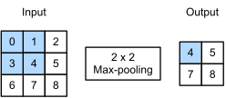
Max pooling takes the maximum value in each local window.
For an input \(X\), a pooling window of size \(K_h\times K_w\) can be written as:
Max pooling can usually be understood as retaining the strongest activation in a local region. If a convolutional channel is detecting vertical edges, for example, max pooling preserves the response as long as one position in the window produces a strong activation.
This also makes the feature less sensitive to small changes in position. Suppose the same high response moves from the left side of a window to the right side. As long as it remains within the same pooling window, the max-pooling output will not change.
However, this does not mean that CNNs naturally have complete translation invariance. When a feature crosses the boundary of a pooling window, the output may still change substantially. Stride, padding, and other layers in the network also affect the result after a translation. More precisely, pooling only reduces the network’s sensitivity to small local shifts.
5.4.3 Average Pooling: Summarizing the Overall Local Response
Average pooling uses the average value within a local window:
y = F.avg_pool2d(x, kernel_size=2, stride=2)print('Average pooled output:', y[0, 0], sep='\n')
Average pooled output:
tensor([[ 3.5000,  5.5000],
        [11.5000, 13.5000]])
Max pooling and average pooling focus on different information:
Max pooling asks: did a particularly strong response appear in this region?
Average pooling asks: how strong is the overall response in this region?
In early image-classification networks, intermediate layers more commonly use max pooling because it highlights strong responses from local detectors. Average pooling often appears near the end of a network, where it summarizes an entire feature map into a channel vector. The global average pooling discussed later is an example of this approach.
We can intuitively compare how the two pooling operations respond to a local outlier.
Max pooling retains the peak value 9 completely, while average pooling combines the four positions into 3. Neither is absolutely better; they simply encode different ways of summarizing a local region.
5.4.4 The Output Size of a Pooling Layer
The output size of a pooling layer uses the same basic formula as a convolutional layer. Without considering dilation:
If stride < kernel_size, adjacent pooling windows overlap. For example:
kernel_size =3stride =2
This is called overlapping pooling. AlexNet once used this setting, although regular twofold downsampling is more common in modern networks.
In PyTorch, if stride is omitted, pooling defaults to:
stride = kernel_size
Therefore:
nn.MaxPool2d(2)
is equivalent to:
nn.MaxPool2d(kernel_size=2, stride=2)
5.4.5 Implementing Two-Dimensional Pooling from Scratch
Pooling and convolution use the same sliding-window framework. The difference is that the window is no longer multiplied by learnable weights; instead, we directly perform max or mean inside it.
The following implements an educational version of pool2d. To highlight the core computation, it supports NCHW input, integer kernel_size, and stride, but does not yet handle padding or dilation.
def pool2d( x: Tensor, kernel_size: int, stride: int|None=None, mode: Literal['max', 'avg'] ='max',) -> Tensor:"""Apply 2D max or average pooling using explicit windows."""if x.ndim !=4:raiseAssertionError('Input must have shape (N, C, H, W).')if kernel_size <=0:raiseAssertionError('`kernel_size` must be positive.')if stride isNone: stride = kernel_sizeif stride <=0:raiseAssertionError('`stride` must be positive.') batch_size, in_channels, input_h, input_w = x.size() output_h = (input_h - kernel_size) // stride +1 output_w = (input_w - kernel_size) // stride +1if output_h <=0or output_w <=0:raiseAssertionError('`kernel_size` must not be larger than the input.') output = x.new_empty(batch_size, in_channels, output_h, output_w)for i inrange(output_h): h_start = i * stride h_end = h_start + kernel_sizefor j inrange(output_w): w_start = j * stride w_end = w_start + kernel_size window = x[:, :, h_start:h_end, w_start:w_end]if mode =='max': output[:, :, i, j] = window.amax(dim=(-2, -1))elif mode =='avg': output[:, :, i, j] = window.mean(dim=(-2, -1))else:raiseNotImplementedError(f'Pooling mode `{mode}` is not implemented.')return output
Is max pooling matches? True
Is avg pooling matches? True
This implementation also illustrates an easily overlooked fact: pooling processes each sample and each channel independently; it does not mix information between channels. If the input has shape \((N,C,H,W)\), pooling changes only \(H\) and \(W\), while the number of output channels remains \(C\). This differs from convolution: an ordinary convolution can change not only the spatial dimensions but also the number of channels through different kernels.
5.4.6 Padding Is Not Exactly the Same in MaxPool and AvgPool
Pooling can also use padding, but its boundary semantics deserve separate attention.
For max pooling, conceptually the padding region does not use ordinary 0s in the maximum comparison. It uses negative infinity instead. This ensures that even when the input contains negative values, the added boundary cannot incorrectly become the maximum.
For average pooling, whether the padding region participates in the divisor is controlled by count_include_pad. By default, it is True, meaning that the added zeros from padding are included in the denominator of the average.
Include padding in divisor:
tensor([[0.2500, 0.5000, 0.2500],
        [0.5000, 1.0000, 0.5000],
        [0.2500, 0.5000, 0.2500]])
Exclude padding from divisor:
tensor([[1., 1., 1.],
        [1., 1., 1.],
        [1., 1., 1.]])
In most basic CNNs, pooling directly uses kernel_size=2, stride=2, padding=0, so these boundary details do not need to be handled often. However, understanding them helps explain why apparently identical padding can produce different results in max pooling and average pooling.
5.4.7 How Pooling Backpropagates
Pooling has no learnable parameters, but it still lies within the computation graph, so gradients must pass through the pooling operation during backpropagation.
For max pooling, the output comes only from the maximum element in the window, so during backpropagation, the gradient is passed only to the position containing the maximum. The gradients at all other positions are 0.
x = torch.tensor([[[[1.0, 3.0], [2.0, 4.0]]]], requires_grad=True)y = F.max_pool2d(x, kernel_size=2)y.backward()print('Max pooled value:', y.item())print('Gradient with respect to input:', x.grad[0, 0], sep='\n')
Max pooled value: 4.0
Gradient with respect to input:
tensor([[0., 0.],
        [0., 1.]])
For average pooling, the output is the average of all elements in the window, so the gradient is distributed evenly among every position in the window.
x = torch.tensor([[[[1.0, 3.0], [2.0, 4.0]]]], requires_grad=True)y = F.avg_pool2d(x, kernel_size=2)y.backward()print('Average pooled value:', y.item())print('Gradient with respect to input:', x.grad[0, 0], sep='\n')
Average pooled value: 2.5
Gradient with respect to input:
tensor([[0.2500, 0.2500],
        [0.2500, 0.2500]])
The gradient of max pooling is relatively sparse, while average pooling sends a gradient to every local position. This is an important difference between the two operations during training.
5.4.8 Adaptive Pooling: Specifying the Output Size Directly
Ordinary pooling requires kernel_size and stride, and the output size is determined by the input size and these hyperparameters. Sometimes, however, we care more about the desired final output size and do not want to manually calculate window parameters for different input sizes.
The interface for adaptive pooling is the opposite: it directly receives the target output size and automatically determines how to divide the input regions.
For example:
nn.AdaptiveAvgPool2d(1)
summarizes the entire feature map in each channel into one value. Whether the input spatial size is \(7\times 7\), \(14\times 14\), or \(32\times 20\), the output spatial size is always \(1\times 1\).
adaptive_pool = nn.AdaptiveAvgPool2d(1)for shape in [(2, 64, 7, 7), (2, 64, 14, 14), (2, 64, 10, 16)]: x = torch.randn(shape) y = adaptive_pool(x)print(f'{shape} -> {y.shape}')
It does not mix different channels; it only averages all spatial positions within each channel.
x = torch.randn(2, 3, 5, 7)actual = x.mean(dim=(-2, -1), keepdim=True)expected = F.adaptive_avg_pool2d(x, output_size=(1, 1))flag = torch.allclose(actual, expected)print('Is global average pooling matches manual mean?', flag)
Is global average pooling matches manual mean? True
Global average pooling is very common in modern classification networks. Suppose the output of the final convolutional stage is:
\[
(N,C,H,W)
\]
After global average pooling, it becomes:
\[
(N,C,1,1)
\]
and is then flattened into:
\[
(N,C)
\]
The classification head then only needs to receive \(C\) channel features and no longer depends on fixed \(H\) and \(W\). Compared with flattening the entire feature map and then connecting it to a large fully connected layer, this usually reduces the number of parameters substantially.
NiN explicitly introduced global average pooling into CNN architecture design. GoogLeNet and many later classification networks continued this idea. We will encounter it again when discussing these classic architectures in the next chapter.
5.4.9 Pooling and Strided Convolution
Pooling is not the only way to downsample. A convolutional layer can also reduce the spatial dimensions while extracting features simply by setting stride > 1. For example, both of the following modules transform a \(32\times 32\) input into \(16\times 16\):
However, the two operations do not perform the same job.
Max pooling:
Has no learnable parameters;
Processes each channel independently;
Usually does not change the number of channels;
Uses a fixed maximum-value rule to summarize local information.
Strided convolution:
Contains learnable weights;
Can mix input channels;
Can change both the spatial dimensions and the number of channels at the same time;
Learns the downsampling rule from the data.
Therefore, many modern architectures reduce explicit pooling and instead use strided convolution to downsample between stages. Pooling has not disappeared, however: global average pooling is still widely used in classification heads, and max pooling still appears in some stems or specific network designs.
It is not accurate to say simply that strided convolution is always better than pooling. More precisely, they provide two different inductive biases. Pooling uses a fixed, parameter-free local aggregation rule, while strided convolution uses a learnable feature transformation to perform downsampling.
It is important to note that downsampling necessarily loses some details because it reduces the number of spatial positions. For image classification, this is usually acceptable because the task cares more about what appears in the image than about the exact output at every pixel. For tasks requiring spatial precision, such as semantic segmentation, object detection, and image generation, downsampling too early or too aggressively may lose boundary and small-object information. Therefore, these models often need to:
Preserve higher-resolution feature maps;
Use features at multiple scales;
Restore spatial dimensions through upsampling;
Use skip connections to pass shallow details forward.
This is also why deconvolution and other upsampling operations are not developed in the main classification-CNN path of this chapter. They are primarily used to restore low-resolution features to a high-resolution space, and it is more natural to discuss them systematically later when introducing AutoEncoders, U-Net, or generative models.
5.4.10 Summary
This section discussed the most common spatial downsampling methods in CNNs.
Max pooling retains the maximum response in each local window:
\[
Y_{i,j} = \max X_{\text{window}}
\]
Average pooling retains the local average response:
Neither operation mixes channels or contains learnable parameters. kernel_size determines the local aggregation range, stride determines the spacing between output positions, and the output size uses the same basic formula as convolution.
Adaptive pooling does not directly specify the window size; instead, it specifies the target output size. In particular:
nn.AdaptiveAvgPool2d((1, 1))
performs global average pooling in each channel, reducing any spatial size to \(1\times 1\) and making the classification head independent of a fixed input resolution.
Finally, both pooling and strided convolution can perform downsampling, but the former uses a fixed rule while the latter uses learnable weights. Modern CNNs choose between them according to the architectural requirements, and may also use both at different locations.
At this point, we have mastered the main modules that make up a basic CNN: convolution extracts local features, activation functions provide nonlinearity, and pooling or strided convolution reduces the spatial resolution. The next section will connect these modules to build and train a complete image-classification CNN.
References
Zhang, Aston, Zachary C. Lipton, Mu Li, and Alexander J. Smola. 2023. Dive into Deep Learning. Cambridge University Press. https://D2L.ai.