Momentum addresses the direction problem: the gradient of the current mini-batch may be noisy, so instead of trusting only the current gradient, we refer to the trend over a period of time in the past. Therefore, momentum can make gradient descent more inertial, accelerate training, and reduce oscillation.
However, there is another problem here that has not been solved:
All parameters still share the same learning rate.
In basic SGD and momentum, the learning rate \(\eta\) is a global scalar. Whether one parameter often has large gradients or another parameter has consistently small gradients, they both use the same learning rate.
This is usually not a big problem in simple models, but in neural networks, the gradient scales of different parameters may differ greatly. Some parameters receive relatively large gradients at every step, while some parameters are updated only occasionally. If all parameters use the same learning rate, a conflict appears:
If the learning rate is too large, parameters with large gradients may update too aggressively;
If the learning rate is too small, parameters with small gradients or sparse updates may learn too slowly.
Adagrad (Duchi et al. 2011) is designed to solve exactly this problem. Its idea is very direct:
Do not let all parameters share the same learning rate. Instead, automatically adjust the effective learning rate of each parameter according to the magnitude of its past gradients.
from collections.abc import Iterablefrom typing import overrideimport dnnlpyimport dnnlpy.optim as doptimport matplotlib.pyplot as pltimport torchimport torch.nn as nnimport torch.nn.functional as Fimport torch.optim as optimfrom torch import Tensordnnlpy.set_matplotlib_format('svg')print('PyTorch version:', torch.__version__)
PyTorch version: 2.14.0+cpu
4.3.1 Why Might One Learning Rate Not Be Enough?
First consider a two-dimensional parameter:
\[
\theta = (\theta_1, \theta_2)
\]
Suppose that during training, the gradient of \(\theta_1\) is often large, while the gradient of \(\theta_2\) is often small. If we use ordinary SGD:
\[
\theta_{t+1} = \theta_t - \eta g_t
\]
then both parameters use the same learning rate \(\eta\).
For \(\theta_1\), because the gradient is already large, multiplying it by the same learning rate may produce an update that is too large, which can easily cause oscillation. For \(\theta_2\), because the gradient is already small, multiplying it by the same learning rate may produce an update that is too small, making learning slow. This shows that the problem is not necessarily in the gradient direction itself, but in the fact that different parameters have different gradient scales. A global learning rate has difficulty taking care of all parameters at the same time.
A more typical example comes from sparse features.
Suppose we are training a model with word embeddings. Common words appear frequently, so their corresponding embeddings are updated frequently; rare words appear only rarely, so their corresponding embeddings are updated only in a small number of batches. If all embedding parameters use the same learning rate, then the parameters of common words will be updated many times, while the parameters of rare words may not move for a long time.
So intuitively, we may want:
Parameters that are updated frequently to move more cautiously later;
Parameters that are updated rarely to take relatively larger steps when they appear.
This is the core motivation of Adagrad.
4.3.2 The Core Idea of Adagrad
The full name of Adagrad is Adaptive Gradient Algorithm(Duchi et al. 2011). Its core is to maintain a historical sum of squared gradients for each parameter.
Suppose the gradient at step \(t\) is:
\[
g_t = \nabla_\theta L_t(\theta_t)
\]
Adagrad maintains a variable \(s_t\) with the same shape as the parameter:
\[
s_t = s_{t-1} + g_t^2
\]
Here the square is an element-wise square. If \(\theta\) is a vector, then \(g_t^2\) is also computed element-wise.
Then Adagrad uses \(s_t\) to scale the current gradient:
where \(\epsilon\) is a very small constant used to avoid a zero denominator.
This formula looks a little more complicated than SGD, but the intuition is very simple.
For a certain parameter, if it often had large gradients in the past, then the corresponding \(s_t\) will become large. After the denominator becomes larger, the effective update step of this parameter becomes smaller. For another parameter, if it was rarely updated in the past, or if its gradients were always small, then the corresponding \(s_t\) is relatively small. With a smaller denominator, this parameter has a relatively larger effective learning rate.
In other words, Adagrad no longer uses the same effective learning rate for all parameters. Instead, it gives each parameter its own scaling factor:
\[
\frac{\eta}{\sqrt{s_t}+\epsilon}
\]
So Adagrad can be understood as:
According to the accumulated magnitude of each parameter’s past gradients, automatically reduce the learning rate of parameters that have often been updated by large amounts.
4.3.3 Understanding Adagrad Through the Effective Learning Rate
To see this more clearly, let us split the Adagrad update formula apart.
can be seen as the effective learning rate of each parameter at step \(t\).
Since \(s_t\) is the accumulated sum of historical squared gradients:
\[
s_t = \sum_{i=1}^{t} g_i^2
\]
\(s_t\) only increases and does not decrease. Therefore, the effective learning rate \(\eta_t\) keeps decreasing during training.
This is exactly the characteristic of Adagrad:
It automatically lowers the learning rate of frequently updated parameters;
It allows sparse parameters to retain relatively large updates when they appear;
But the longer training continues, the effective learning rates of all parameters gradually decrease.
The first two characteristics are advantages, while the last one becomes its main problem.
In the early stage of training, Adagrad’s adaptive scaling is very helpful. It can quickly suppress directions with large gradients, making training more stable. However, in the later stage of training, if \(s_t\) has already accumulated to a large value, the denominator becomes very large, and the effective learning rate may become extremely small. The parameters almost stop moving, and training may stop too early.
This is also why later RMSprop and Adadelta continue to modify Adagrad: they want to keep the idea of adaptive scaling by parameter, but they do not want the historical sum of squared gradients to accumulate without bound. Otherwise, training becomes overly conservative in the later stage.
4.3.4 Comparing the Trajectories of Adagrad and SGD
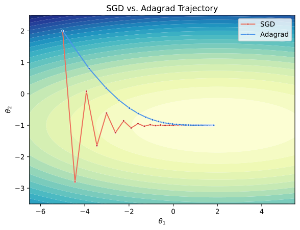
We first use a simple two-dimensional function to observe the behavior of Adagrad:
\[
L(x, y) = 0.1 (x - 2)^2 + 2.0 (y + 1)^2
\]
This function is steeper in the \(y\) direction and flatter in the \(x\) direction. On this narrow loss surface, ordinary SGD may need a relatively small learning rate to remain stable. If the learning rate is slightly too large, the steep direction can easily oscillate.
Adagrad adjusts the step size according to the magnitude of past gradients in each direction. Since the gradient in the \(y\) direction is often larger, its effective learning rate decreases faster. Since the gradient in the \(x\) direction is smaller, it retains a relatively larger effective learning rate.
We can see that the SGD trajectory oscillates more in the \(y\) direction, while the Adagrad trajectory converges faster to a better point. This is because Adagrad automatically lowers the effective learning rate in the \(y\) direction, making the updates more cautious. However, in the later stage of training, Adagrad’s update step becomes very small, and the parameters almost stop moving.
4.3.5 Visualizing the Effective Learning Rate of Adagrad
The most important thing to pay attention to in Adagrad is not the parameter update formula itself, but the effective learning rate it produces.
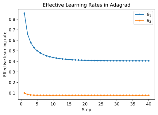
We can plot the effective learning rates of the two parameters in the example above:
lr_history = torch.stack([lr[0] for lr in optimizer2.effective_lrs])steps = torch.arange(1, lr_history.size(0) +1)fig = plt.figure(2, figsize=(6, 4))ax = fig.add_subplot(1, 1, 1)ax.plot(steps, lr_history[:, 0], marker='o', markersize=3)ax.plot(steps, lr_history[:, 1], marker='o', markersize=3)ax.set_xlabel('Step')ax.set_ylabel('Effective learning rate')ax.legend([r'$\theta_1$', r'$\theta_2$'])ax.set_title('Effective Learning Rates in Adagrad')plt.show()
From the figure, we can see that different parameters do not have the same effective learning rate. Because each parameter has its own historical sum of squared gradients, they are scaled to different degrees. At the same time, the effective learning rates as a whole gradually decrease during training. The reason is simple:
\[
s_t = s_{t-1} + g_t^2
\]
As long as the gradient is not strictly 0, \(s_t\) continues to increase. The larger the denominator, the smaller the effective learning rate. This also shows that Adagrad’s adaptivity comes with a cost: it makes updates conservative by continuously accumulating historical gradients, but this accumulation process never forgets the past.
4.3.6 Why Is Adagrad Suitable for Sparse Features?
One of the most classic advantages of Adagrad is that it is suitable for handling sparse features.
Sparse features mean that only a small subset of parameters is updated during each training step. For example, in natural language processing, if a model has a large embedding table, then only a small subset of tokens appears in one mini-batch. Only the embeddings corresponding to these tokens receive gradients, while the gradients of the embeddings for other tokens are 0.
For frequently appearing tokens, their embeddings are updated often. Adagrad gradually increases the corresponding \(s_t\) of these parameters, thereby lowering their effective learning rates. For rarely appearing tokens, their embeddings rarely receive nonzero gradients. The corresponding \(s_t\) grows slowly, so once they appear, they can still retain a relatively large effective learning rate.
This leads to a very natural effect:
Frequently appearing parameters learn more and more cautiously, while rare but important parameters do not become completely unable to learn just because the global learning rate is too small.
This is also why Adagrad is attractive in some sparse-feature tasks.
However, for modern deep neural networks, especially large models that require long training, Adagrad’s continuously decaying learning rate problem can be quite obvious. In the later stage of training, \(s_t\) may already be very large, causing the update step to become too small.
Therefore, Adagrad is more like the starting point of adaptive learning rate methods, rather than the most commonly used default optimizer in modern deep learning.
4.3.7 The Relationship Between Adagrad, SGD, and Momentum
At this point, we can compare SGD, momentum, and Adagrad together.
The problem with SGD is that each step only looks at the current gradient, and all parameters share the same learning rate.
Momentum improves the first part. It no longer looks only at the current gradient. Instead, it accumulates past gradient directions, making the update more inertial:
\[
v_t = \beta v_{t-1} + g_t
\]
Adagrad improves the second part. It still uses the current gradient direction, but adjusts the effective learning rate according to the magnitude of each parameter’s past gradients:
Momentum focuses on smoothing and accelerating the direction;
Adagrad focuses on scaling the step size of different parameters.
These two ideas will later merge again in Adam. On one hand, Adam maintains the first moment of gradients like momentum; on the other hand, it maintains an exponential moving average of squared gradients like RMSprop, which is used for adaptive scaling.
However, before discussing Adam, let us first talk about RMSprop. It starts from the main problem of Adagrad:
Since the historical sum of squared gradients keeps accumulating and makes the learning rate smaller and smaller, can we let the optimizer forget gradients from too long ago?
4.3.8 Summary
In this section, we started from the problem that SGD and momentum still share a global learning rate, and introduced Adagrad.
The core idea of Adagrad is to maintain a historical sum of squared gradients for each parameter:
\[
s_t = s_{t-1} + g_t^2
\]
Then this accumulated quantity is used to scale the current gradient:
In this way, parameters with larger past gradients obtain smaller effective learning rates; parameters with smaller past gradients or parameters that are rarely updated retain relatively larger effective learning rates.
Adagrad is intuitive and effective, especially in sparse-feature scenarios. For the first time, it clearly reflects an important idea: an optimizer does not necessarily need to use the same learning rate for all parameters. However, Adagrad also has an obvious problem: the historical sum of squared gradients only increases and never decreases. Therefore, the effective learning rate keeps decreasing, and training may become overly conservative in the later stage.
In the next section, we will see that RMSprop and Adadelta continue improving along exactly this problem. They keep Adagrad’s idea of adaptive scaling, but replace “accumulating all historical squared gradients” with “an exponential moving average of recent squared gradients.”
References
Duchi, John, Elad Hazan, and Yoram Singer. 2011. “Adaptive Subgradient Methods for Online Learning and Stochastic Optimization.”Journal of Machine Learning Research 12 (61): 2121–59. http://jmlr.org/papers/v12/duchi11a.html.