import math

import dnnlpy
import dnnlpy.nn as dnn
import torch
import torch.nn as nn
import torchinfo
from torch import Tensor

print('PyTorch version:', torch.__version__)
PyTorch version: 2.14.0+cpu
The previous sections introduced convolution, pooling, downsampling, and the training process for a complete CNN separately. At this point, we know that an image-classification network can consist of several convolutional blocks and a classification head, but we still need a concrete architecture to show how these components should be arranged and how the channel counts and spatial dimensions should change.
LeNet-5 is an ideal classic CNN to use as a starting point. Its structure is not complex, yet it already contains the basic pattern that image-classification networks continued to use for many years: first extract local features through convolutional layers, then gradually reduce the spatial resolution through pooling, and finally use fully connected layers to perform classification.
Its overall structure can be summarized as:
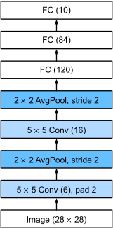
Today’s CNNs are much deeper than LeNet and also use ReLU, batch normalization, residual connections, and more sophisticated downsampling methods. But if we set aside these later improvements, many modern classification networks can still be understood as answering the same question:
How can a high-resolution, low-semantic pixel grid be gradually transformed into a low-resolution, high-semantic feature representation?
This section will first reconstruct the basic structure of LeNet-5 and then implement a version using modern PyTorch conventions that better fits current training practices. The focus is not on reproducing every historical detail, but on understanding why LeNet became a structural template for later CNNs.
import math
import dnnlpy
import dnnlpy.nn as dnn
import torch
import torch.nn as nn
import torchinfo
from torch import Tensor
print('PyTorch version:', torch.__version__)PyTorch version: 2.14.0+cpuBefore LeNet appeared, handwritten-digit recognition often relied on manually designed image features. Researchers first had to decide which edges, strokes, or geometric shapes to extract, and then pass those features to a classifier.
CNNs changed this process. Instead of relying on manually specified features, the network directly learns a series of representations from pixels, combining them layer by layer:
pixels
  ↓
edges and simple strokes
  ↓
local stroke combinations
  ↓
digit-level representation
  ↓
class prediction
LeNet’s importance lies not only in using convolution, but also in combining several key ideas into an end-to-end trainable system:
Therefore, LeNet can be regarded as an early representative of the shift from manually designed features to automatic feature learning with neural networks.
LeNet-5 usually accepts a single-channel image of size \(32\times 32\). For the \(28\times 28\) MNIST dataset, we can first pad the image with zeros on all sides to make it \(32\times 32\).
The shape changes in the classic architecture are:
Input:        (N,   1, 32, 32)
Conv 5x5:     (N,   6, 28, 28)
Pool 2x2:     (N,   6, 14, 14)
Conv 5x5:     (N,  16, 10, 10)
Pool 2x2:     (N,  16,  5,  5)
Conv 5x5:     (N, 120,  1,  1)
Flatten:      (N, 120)
Linear:       (N, 84)
Output:       (N, 10)
The first convolution does not use padding, so the spatial dimensions change from \(32\times 32\) to:
\[ 32 - 5 + 1 = 28 \]
Then, \(2\times 2\) pooling halves both the height and width:
\[ 28\times 28 \rightarrow 14\times 14 \]
The second convolution again uses a \(5\times 5\) kernel:
\[ 14 - 5 + 1 = 10 \]
After another pooling operation, the feature map is \(5\times 5\). The final \(5\times 5\) convolution covers the entire spatial region, so:
\[ 5 - 5 + 1 = 1 \]
This produces an output with shape (N, 120, 1, 1). After flattening the spatial dimensions, each image is represented by a 120-dimensional vector.
Some connectivity patterns, activation functions, and loss functions in the original LeNet-5 are not exactly the same as those in commonly used PyTorch implementations today. In teaching, we usually retain the overall structure while using standard fully connected convolutions, modern activation functions, and cross-entropy loss.
We first implement LeNet according to the classic shape changes. To stay closer to the original model, we use Tanh and average pooling, while the output layer still returns logits directly so that it can be used with the modern nn.CrossEntropyLoss.
class LeNet5(nn.Module):
    """A practical implementation of the classic LeNet-5 architecture."""

    def __init__(self, num_classes: int = 10):
        super().__init__()
        self.features = nn.Sequential(
            dnn.Conv2d(1, 6, kernel_size=5),
            dnn.Tanh(),
            dnn.AvgPool2d(kernel_size=2),
            dnn.Conv2d(6, 16, kernel_size=5),
            dnn.Tanh(),
            dnn.AvgPool2d(kernel_size=2),
            dnn.Conv2d(16, 120, kernel_size=5),
            dnn.Tanh(),
        )
        self.classifier = nn.Sequential(
            dnn.Flatten(),
            dnn.Linear(120, 84),
            dnn.Tanh(),
            dnn.Linear(84, num_classes),
        )

    def forward(self, x: Tensor) -> Tensor:
        x = self.features(x)
        x = self.classifier(x)
        return x


model = LeNet5(num_classes=10)
x = torch.randn(8, 1, 32, 32)
logits = model(x)

print(model, end='\n\n')
print('Input shape:', x.shape)
print('Output shape:', logits.shape)
LeNet5(
(features): Sequential(
(0): Conv2d(1, 6, kernel_size=(5, 5), stride=(1, 1))
(1): Tanh()
(2): AvgPool2d(kernel_size=2, stride=2, padding=0)
(3): Conv2d(6, 16, kernel_size=(5, 5), stride=(1, 1))
(4): Tanh()
(5): AvgPool2d(kernel_size=2, stride=2, padding=0)
(6): Conv2d(16, 120, kernel_size=(5, 5), stride=(1, 1))
(7): Tanh()
)
(classifier): Sequential(
(0): Flatten(start_dim=1, end_dim=-1)
(1): Linear(in_features=120, out_features=84, bias=True)
(2): Tanh()
(3): Linear(in_features=84, out_features=10, bias=True)
)
)
Input shape: torch.Size([8, 1, 32, 32])
Output shape: torch.Size([8, 10])The model output has shape (8, 10). The 10 values are not probabilities; they are the logits for the 10 classes. During training, they can be passed directly to:
loss_fn = nn.CrossEntropyLoss()CrossEntropyLoss internally performs log_softmax and the negative log-likelihood calculation, so the final layer of the model does not need an additional Softmax.
The number of parameters in a convolutional layer is:
\[ C_{\text{out}} \left( C_{\text{in}} K_h K_w + 1 \right) \]
The final 1 corresponds to the bias for each output channel.
For example, the number of parameters in the first convolutional layer is:
\[ 6 \times (1 \times 5 \times 5 + 1) = 156 \]
The number of parameters in the second convolutional layer is:
\[ 16 \times (6 \times 5 \times 5 + 1) = 2416 \]
Although convolutional layers reuse kernels across the entire image, the same kernel shares parameters at every spatial position. Therefore, the number of parameters depends only on the input channels, output channels, and kernel size, not on how many times the kernel slides.
The following counts the parameters in each learnable layer.
summary = torchinfo.summary(model, input_size=(8, 1, 32, 32))
print(summary)
==========================================================================================
Layer (type:depth-idx) Output Shape Param #
==========================================================================================
LeNet5 [8, 10] --
├─Sequential: 1-1 [8, 120, 1, 1] --
│ └─Conv2d: 2-1 [8, 6, 28, 28] 156
│ └─Tanh: 2-2 [8, 6, 28, 28] --
│ └─AvgPool2d: 2-3 [8, 6, 14, 14] --
│ └─Conv2d: 2-4 [8, 16, 10, 10] 2,416
│ └─Tanh: 2-5 [8, 16, 10, 10] --
│ └─AvgPool2d: 2-6 [8, 16, 5, 5] --
│ └─Conv2d: 2-7 [8, 120, 1, 1] 48,120
│ └─Tanh: 2-8 [8, 120, 1, 1] --
├─Sequential: 1-2 [8, 10] --
│ └─Flatten: 2-9 [8, 120] --
│ └─Linear: 2-10 [8, 84] 10,164
│ └─Tanh: 2-11 [8, 84] --
│ └─Linear: 2-12 [8, 10] 850
==========================================================================================
Total params: 61,706
Trainable params: 61,706
Non-trainable params: 0
Total mult-adds (Units.MEGABYTES): 3.38
==========================================================================================
Input size (MB): 0.03
Forward/backward pass size (MB): 0.42
Params size (MB): 0.25
Estimated Total Size (MB): 0.70
==========================================================================================From the parameter statistics, the layer with the most parameters in LeNet-5 is the final convolutional layer, C5, rather than an explicitly fully connected layer. C5 uses a \(5\times 5\) kernel to map a feature map of size \(16\times 5\times 5\) to \(120\times 1\times 1\). Thus, although it is structurally a convolutional layer, every output unit is connected to all features in the preceding layer, making it functionally very similar to a fully connected layer.
Therefore, more precisely, most of LeNet-5’s parameters are concentrated in the densely connected classification module at the back of the network, rather than in the local feature-extraction layers at the front. Later architectures such as NiN and GoogLeNet introduced global average pooling so that each channel could be directly aggregated into a spatial average, reducing their dependence on such parameter-heavy dense classification layers. We will discuss this further in the next chapter.
If we redesigned a small CNN of comparable size today, we would usually not copy every detail of LeNet. A more modern version might make the following changes:
Tanh with ReLU;The following gives a modernized LeNet-style model.
class ModernLeNet5(nn.Module):
    """A modernized LeNet-style CNN with adaptive pooling."""

    def __init__(self, num_classes: int = 10) -> None:
        super().__init__()
        self.features = nn.Sequential(
            dnn.Conv2d(1, 16, kernel_size=3, padding=1),
            dnn.ReLU(),
            dnn.MaxPool2d(kernel_size=2),
            dnn.Conv2d(16, 32, kernel_size=3, padding=1),
            dnn.ReLU(),
            dnn.MaxPool2d(kernel_size=2),
        )
        self.pool = dnn.AdaptiveAvgPool2d(1)
        self.flatten = dnn.Flatten()
        self.classifier = dnn.Linear(32, num_classes)

    def forward(self, x: Tensor) -> Tensor:
        x = self.features(x)
        x = self.pool(x)
        x = self.flatten(x)
        x = self.classifier(x)
        return x


model = ModernLeNet5(num_classes=10)
summary = torchinfo.summary(model, input_size=(8, 1, 32, 32))
print(summary)
==========================================================================================
Layer (type:depth-idx) Output Shape Param #
==========================================================================================
ModernLeNet5 [8, 10] --
├─Sequential: 1-1 [8, 32, 8, 8] --
│ └─Conv2d: 2-1 [8, 16, 32, 32] 160
│ └─ReLU: 2-2 [8, 16, 32, 32] --
│ └─MaxPool2d: 2-3 [8, 16, 16, 16] --
│ └─Conv2d: 2-4 [8, 32, 16, 16] 4,640
│ └─ReLU: 2-5 [8, 32, 16, 16] --
│ └─MaxPool2d: 2-6 [8, 32, 8, 8] --
├─AdaptiveAvgPool2d: 1-2 [8, 32, 1, 1] --
├─Flatten: 1-3 [8, 32] --
├─Linear: 1-4 [8, 10] 330
==========================================================================================
Total params: 5,130
Trainable params: 5,130
Non-trainable params: 0
Total mult-adds (Units.MEGABYTES): 10.82
==========================================================================================
Input size (MB): 0.03
Forward/backward pass size (MB): 1.57
Params size (MB): 0.02
Estimated Total Size (MB): 1.63
==========================================================================================Because it uses AdaptiveAvgPool2d(1), this model can accept inputs with different spatial dimensions. In contrast, the classic LeNet’s fully connected layer expects the output after exactly two convolution-and-pooling stages to have shape (120, 1, 1), so it depends more strongly on the input size.
Of course, the modern version is not necessarily better than the classic one. LeNet’s design is very suitable for small image-classification tasks such as MNIST, while the modernized changes are mainly intended to accommodate larger and more complex image datasets.
In classic LeNet, the final convolution maps (N, 16, 5, 5) to (N, 120, 1, 1). Since the kernel is also \(5\times 5\), it covers the entire input feature map spatially. At this point, the convolutional layer is very similar to a fully connected layer. For each sample, every output channel uses a set of weights with size:
\[ 16\times 5\times 5 \]
to compute a weighted sum over the entire input feature map.
We can verify that a convolution covering the entire spatial region and a linear layer can produce the same result.
x = torch.randn(3, 16, 5, 5)
conv = nn.Conv2d(16, 120, kernel_size=5)
linear = nn.Linear(16 * 5 * 5, 120)

with torch.no_grad():
    linear.weight.copy_(conv.weight.reshape(120, -1))
    linear.bias.copy_(conv.bias)

conv_output = conv(x).flatten(start_dim=1)
linear_output = linear(x.flatten(start_dim=1))

max_diff = (conv_output - linear_output).abs().max()
print('Maximum difference:', max_diff.item())
Maximum difference: 1.0728836059570312e-06This shows that convolutional and linear layers are not completely different types of operations. A convolutional layer is fundamentally also a linear transformation, but it adds image-suitable structural constraints through local connectivity and weight sharing. When the kernel covers the entire spatial region and computes only one output position, this spatial sharing no longer has an effect, and the operation degenerates into an ordinary linear layer.
LeNet’s specific scale is very small by today’s standards, but its structural ideas remain important.
First, it established the basic division of labor between a “feature extractor + classification head.” The convolutional layers at the front convert pixels into features, while the classifier at the back produces classes based on those features.
Second, it demonstrated a typical shape change in CNNs: the spatial dimensions gradually decrease while the number of channels gradually increases. Although later models such as AlexNet, VGG, and ResNet are much larger, they still follow this overall trend.
Finally, it showed that image features do not necessarily need to be designed by hand. By combining local connectivity, weight sharing, and backpropagation, a network can learn features suitable for a task directly from data.
However, LeNet also left several problems unresolved:
These questions drove the development of later CNN architectures. AlexNet brought CNNs to large-scale image classification, VGG explored building deeper networks with small kernels, NiN and GoogLeNet introduced \(1\times 1\) convolutions and more flexible channel transformations, ResNet made very deep networks easier to optimize through residual connections, and MobileNet and EfficientNet paid more attention to computational efficiency and model scaling.
LeNet is therefore not merely a classic model to memorize. It is more like the starting point for CNN architecture design:
First extract spatial features layer by layer with convolution, then pass the final representation to a classifier.
Using LeNet, this section combined the convolution, activation, pooling, and fully connected layers introduced earlier into a complete classic CNN.
The core structure of LeNet is:
Conv → Pool → Conv → Pool → Conv/Flatten → Linear → OutputDuring this process, the spatial dimensions gradually decrease and the number of channels gradually increases, transforming local pixels into high-level features suitable for classification. It also demonstrates the basic division of labor between a convolutional feature extractor and a fully connected classification head, and explains why modern networks later began using global average pooling and more flexible classification heads.
At this point, the basic components of CNNs are essentially complete. The next chapter will no longer introduce operators one by one. Instead, following the development of CNN architectures, it will discuss how researchers continuously improved image feature extractors through deeper networks, smaller kernels, \(1\times 1\) convolutions, multi-scale branches, residual connections, and separable convolutions.