3.4 Forward and Backward Propagation of Linear Layers
Author
jshn9515
Published
2026-06-07
Modified
2026-06-07
In the previous sections, we discussed several key components in an MLP:
Linear transformations map inputs into a new feature space;
Activation functions introduce nonlinearity;
Softmax cross entropy converts the final logits into a loss and provides the starting point for backpropagation.
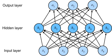
Now we return to the most fundamental and most common module in an MLP: the linear layer. Before going into the specific formulas, let us first look at where linear layers appear in the overall structure of an MLP. In practice, we usually add an activation function after each hidden layer, but we will temporarily ignore that here.
As shown in the figure, adjacent layers in an MLP are usually fully connected. Each edge corresponds to a learnable weight, and the overall computation from one layer to the next can be written as a linear transformation.
For a two-layer MLP, the linear layer appears twice:
\[
\begin{align}
H &= XW_1 + b_1 \\
Y &= HW_2 + b_2
\end{align}
\]
Although their input and output dimensions are different, they are essentially doing the same thing:
\[
Y = XW + b
\]
In this section, we will derive the forward and backward propagation of a linear layer, and then implement a reusable Linear class with NumPy. Later, when we handwrite a complete MLP, we will directly use this module.
Therefore, the role of a linear layer is to map each sample from a \(D_{\text{in}}\)-dimensional space to a \(D_{\text{out}}\)-dimensional space.
3.4.2 Backward Propagation of a Linear Layer
When training a neural network, forward propagation produces the loss \(L\), while backward propagation needs to compute the gradient of the loss with respect to each parameter.
For a linear layer:
\[
Y = XW + b
\]
During backpropagation, we receive the upstream gradient from the next layer:
\[
G = \frac{\partial L}{\partial Y}
\]
Its shape is the same as \(Y\):
\[
G \in \mathbb{R}^{B \times D_{\text{out}}}
\]
The linear layer needs to compute three things from this upstream gradient:
The gradient of the loss with respect to the input: \(\frac{\partial L}{\partial X}\), which is passed further to the previous layer;
The gradient of the loss with respect to the weight: \(\frac{\partial L}{\partial W}\), which is used to update \(W\);
The gradient of the loss with respect to the bias: \(\frac{\partial L}{\partial b}\), which is used to update \(b\).
In other words, the backward method of a linear layer takes \(G\) as input, returns \(\frac{\partial L}{\partial X}\), and also stores \(\frac{\partial L}{\partial W}\) and \(\frac{\partial L}{\partial b}\).
3.4.2.1 Gradient with Respect to the Input
First, let us look at the gradient with respect to the input \(X\). For a batch, the linear layer can be written as:
\[
Y = XW + b
\]
where:
\[
\begin{align}
X &\in \mathbb{R}^{B \times D_{\text{in}}} \\
W &\in \mathbb{R}^{D_{\text{in}} \times D_{\text{out}}} \\
b &\in \mathbb{R}^{D_{\text{out}}} \\
Y &\in \mathbb{R}^{B \times D_{\text{out}}}
\end{align}
\]
The \(j\)-th component of the \(i\)-th output sample can be written as:
Therefore, if we want to know how the \(k\)-th input component \(X_{i,k}\) of the \(i\)-th sample affects the loss, we need to sum its effects over all output dimensions of that sample:
This exactly corresponds to the matrix multiplication:
\[
\frac{\partial L}{\partial W} = X^\top G
\]
with shape:
\[
(D_{\text{in}}, B) @ (B, D_{\text{out}}) = (D_{\text{in}}, D_{\text{out}})
\]
Therefore, the shape of \(\frac{\partial L}{\partial W}\) is the same as the shape of \(W\).
This point is important: the gradient of a parameter must have the same shape as the parameter itself. Otherwise, we cannot use it to update the parameter.
3.4.2.3 Gradient with Respect to the Bias
Finally, let us look at the bias \(b\). During forward propagation, the bias is added to the output of every sample:
\[
Y_i = X_i W + b
\]
For the \(j\)-th bias \(b_j\), it affects the \(j\)-th output of all samples in the batch. Therefore:
G = rng.random((B, D_out))dX = G @ W.TdW = X.T @ Gdb = np.sum(G, axis=0)print('dX.shape:', dX.shape)print('dW.shape:', dW.shape)print('db.shape:', db.shape)
dX.shape: (4, 3)
dW.shape: (3, 2)
db.shape: (2,)
The most common mistakes in backpropagation are usually matrix transposes and summation dimensions. Therefore, when implementing a linear layer, it is best to always use shapes to check whether each step is reasonable.
3.4.3 Implementing a Linear Layer with NumPy
Before implementing the Linear layer, we first define a Parameter class to wrap learnable parameters.
This class inherits from NumPy’s ndarray and adds a .grad attribute to store gradients. Its role is similar to nn.Parameter in PyTorch, but without the Autograd part. You do not need to understand the implementation of this class. You only need to know that it is a NumPy array with a gradient attribute.
Now we can wrap the linear layer as a class. It needs to do several things:
Initialize the parameters \(W\) and \(b\);
Compute \(XW + b\) in forward;
Save the input \(X\), because it is needed during backward;
Compute dx, dW, and db in backward.
class Linear(Module):"""Fully connected affine layer for batched NumPy inputs."""def__init__(self, in_features: int, out_features: int):super().__init__()self.in_features = in_featuresself.out_features = out_features weight = rng.standard_normal((in_features, out_features)) weight = weight * math.sqrt(2.0/ in_features) bias = np.zeros(out_features)self.weight = Parameter(weight)self.bias = Parameter(bias)@overridedef forward(self, x: np.ndarray) -> np.ndarray:self.ctx = x # save input for backwardreturn x @self.weight +self.bias@overridedef backward(self, grad: np.ndarray) -> np.ndarray:assertself.ctx isnotNone, 'Must call forward before backward.' x =self.ctx # recover saved inputself.weight.grad = x.T @ grad # dWself.bias.grad = np.sum(grad, axis=0) # dbreturn grad @self.weight.T # dx@overridedef parameters(self) -> Iterator[Parameter]:for value inself.__dict__.values():ifisinstance(value, Parameter):yield valueelifisinstance(value, Module):yieldfrom value.parameters()
Here, grad is the upstream gradient, which is the \(G\) in the derivation above.
When initializing the weight \(W\), we used He initialization:
\[
W \sim \mathcal{N}\left(0, \frac{2}{D_{\text{in}}}\right)
\]
It is often used together with ReLU. Its purpose is to prevent the signal from growing or shrinking too quickly as it propagates between layers. We will not expand on initialization theory here; we will simply use it as a more stable default choice than directly using a standard normal distribution.
We can briefly test whether its shapes are correct:
This shows that the Linear layer can already be used like a real neural network module: it receives inputs during forward propagation, receives upstream gradients during backward propagation, and passes gradients back to the previous layer.
3.4.4 Parameter Updates
The backward method of a linear layer is only responsible for computing gradients. It does not directly update the parameters. Parameter updates are usually handled by an optimizer. The simplest optimizer is SGD:
\[
\begin{align}
W &\leftarrow W - \eta \frac{\partial L}{\partial W} \\
b &\leftarrow b - \eta \frac{\partial L}{\partial b}
\end{align}
\]
where \(\eta\) is the learning rate.
In NumPy, this is:
class SGD(Optimizer):def__init__(self, params: Iterable[Parameter], lr: float=0.1):super().__init__(params)self.lr = lr@overridedef step(self):for p inself.params:if p.grad isNone:continue p -=self.lr * p.grad
Here, the parameters() method returns all learnable parameters of this layer, wrapped with Parameter, namely the weight W and the bias b. If a module contains submodules, then parameters() recursively returns the parameters inside those submodules.
One design principle is very important here:
Forward computes outputs, backward computes gradients, and parameter updates modify parameters according to gradients.
Although these three steps happen consecutively in the training loop, conceptually they should be understood separately.
3.4.5 Summary
In this section, we derived and implemented the forward and backward propagation of a linear layer.
From the implementation perspective, a linear layer needs to save the input during forward, because \(X\) is needed when backward computes \(\frac{\partial L}{\partial W}\). This also reflects a basic rule of backpropagation: each layer saves the necessary information during forward, and uses this information together with the upstream gradient during backward to compute its own gradients.
At this point, we already have the main building blocks of an MLP: linear layers, activation functions, and softmax cross entropy. In the next section, we will put these modules together and build a complete MLP with NumPy.
References
Zhang, Aston, Zachary C. Lipton, Mu Li, and Alexander J. Smola. 2023. Dive into Deep Learning. Cambridge University Press. https://D2L.ai.