3.2 Activation Functions: Adding Nonlinearity to Neural Networks
Author
jshn9515
Published
2026-06-07
Modified
2026-06-08
In the previous section, we saw that if we simply stack multiple linear layers together, the entire model is still equivalent to a single linear layer:
\[
Z = XW' + b'
\]
In other words, even though the number of layers increases, the model is still fundamentally limited to representing linear transformations. To allow neural networks to represent more complex functions, we need to insert nonlinear operations between linear layers. This nonlinear operation is called an activation function.
For a two-layer MLP, we can write:
\[
\begin{align}
H &= XW_1 + b_1 \\
A &= \phi(H) \\
Z &= AW_2 + b_2
\end{align}
\]
Here, \(\phi\) is the activation function. It usually acts element-wise on \(H\), meaning that every element in \(H\) passes through the same function.
In this section, we first introduce several classic activation functions and derive their gradients in backpropagation. We will implement activation functions as standalone modules, each with its own forward and backward, so that they can be directly used in the MLP implementation later.
from typing import overrideimport dnnlpyimport matplotlib.pyplot as pltimport numpy as npfrom dnnlpy.models.mlp import Modulerng = np.random.default_rng(42)dnnlpy.set_matplotlib_format('svg')print('NumPy version:', np.__version__)
NumPy version: 2.5.3
3.2.1 Background: Jacobian Matrix and VJP
Before formally introducing activation functions, let us first fill in a concept that is often overlooked in backpropagation: the Jacobian matrix.
Start with an ordinary single-variable function. Suppose:
\[
y = f(x)
\]
where both \(x\) and \(y\) are scalars. Then the derivative is:
\[
\frac{dy}{dx}
\]
It describes how the output \(y\) changes when the input \(x\) changes slightly.
However, variables in neural networks are usually not scalars, but vectors or matrices. For example, one layer can be viewed as a function from a vector to a vector:
\[
y = f(x), \quad x \in \mathbb{R}^n, \quad y \in \mathbb{R}^m
\]
That is, the input has \(n\) components:
\[
x = [x_1, x_2, \dots, x_n]
\]
and the output has \(m\) components:
\[
y = [y_1, y_2, \dots, y_m]
\]
At this point, we cannot describe the change of \(f\) with just one derivative, because each output \(y_i\) may depend on each input \(x_j\). Therefore, we need to arrange all partial derivatives into a matrix:
This matrix is the Jacobian matrix. Its entry in row \(i\) and column \(j\) represents how much the \(j\)-th input component \(x_j\) affects the \(i\)-th output component \(y_i\).
So why does backpropagation need the Jacobian matrix? Because backpropagation is essentially repeated application of the chain rule in a composite function.
Suppose the loss function \(L\) does not depend directly on \(x\), but depends on \(x\) through an intermediate variable \(y\):
\[
x \rightarrow y = f(x) \rightarrow L
\]
During backpropagation, we usually already know the upstream gradient:
\[
\frac{\partial L}{\partial y}
\]
Now we need to continue propagating backward and compute:
\[
\frac{\partial L}{\partial x}
\]
According to the chain rule, \(\frac{\partial L}{\partial x}\) is made from two parts:
The gradient of \(L\) with respect to \(y\), namely the upstream gradient;
The derivative of \(y\) with respect to \(x\), namely the Jacobian matrix of the current module.
If we view the gradient as a row vector, we can write:
The backward of each module is essentially multiplying the upstream gradient by the Jacobian matrix of the current module.
However, when writing deep learning code in practice, we almost never explicitly construct the full Jacobian matrix. The reason is simple: it is too large. For example, if a function maps a 1000-dimensional vector to another 1000-dimensional vector, the Jacobian matrix is \(1000 \times 1000\), already containing one million elements. For images, sequences, or hidden states in large models, the full Jacobian matrix becomes even larger.
Therefore, what deep learning frameworks actually compute is usually not the full \(J_f(x)\), but the result of multiplying the upstream gradient by the Jacobian matrix:
\[
\frac{\partial L}{\partial y} J_f(x)
\]
This is also called a VJP (vector-Jacobian product). In other words, backpropagation does not care about writing out the entire Jacobian matrix; it cares about efficiently propagating the upstream gradient to the input.
The activation functions we are about to discuss are a good example. Activation functions usually act element-wise:
\[
y_i = \phi(x_i)
\]
The phrase “element-wise” is crucial here: the \(i\)-th output depends only on the \(i\)-th input, and not on any other input component. Therefore:
This is why the backward of an activation function is usually written as:
grad_input = grad_output * local_derivative
Mathematically, this is doing “upstream gradient \(\times\) Jacobian matrix.” In code, because the Jacobian matrix of an element-wise activation function is diagonal, we can implement it efficiently using element-wise multiplication.
3.2.2 What Does an Activation Function Do?
From the previous subsection, we know that the backward of an activation function is not just an arbitrary element-wise multiplication; it is the simplification of a VJP when the Jacobian matrix is diagonal. Now let us return to forward propagation and see why activation functions are placed after linear layers.
Suppose a linear layer outputs a scalar \(h\). Without an activation function, the next layer still receives this linear output:
\[
a = h
\]
If we add an activation function, it becomes:
\[
a = \phi(h)
\]
The role of an activation function can be understood from two perspectives.
First, in forward propagation, an activation function changes the hidden representation. For example, ReLU turns negative numbers into 0 and keeps positive numbers unchanged:
\[
\operatorname{ReLU}(h) = \max(0, h)
\]
This means the hidden layer is no longer just a linear transformation of the input, but has gone through a nonlinear selection. Without such nonlinearity, stacking multiple linear layers is still equivalent to a single linear layer.
Second, in backpropagation, an activation function controls how gradients continue to propagate to the previous layer. In the scalar case, if:
\[
a = \phi(h)
\]
and the upstream gradient is \(\frac{\partial L}{\partial a}\), then by the chain rule:
For the matrix form more commonly used in MLPs, suppose:
\[
H \in \mathbb{R}^{B \times D}, \quad A = \phi(H)
\]
Here, \(B\) is the batch size and \(D\) is the hidden dimension. The activation function acts element-wise, so:
\[
A_{b,d} = \phi(H_{b,d})
\]
If we flatten \(H\) and \(A\) into vectors, then the output at position \((b,d)\) depends only on the input at position \((b,d)\) and not on any other position:
Therefore, the Jacobian matrix of \(A\) with respect to \(H\) is diagonal, and the diagonal elements are the local derivatives at the corresponding positions:
where \(\odot\) denotes element-wise multiplication.
This is also the shared structure of the next three activation functions: first derive the derivative of the scalar function, then use “element-wise operation \(\Rightarrow\) diagonal Jacobian matrix” to write backward as the element-wise product of the upstream gradient and the local derivative.
3.2.3 Sigmoid Activation Function
Sigmoid was a very common activation function in early neural networks:
\[
\sigma(x) = \frac{1}{1 + e^{-x}}
\]
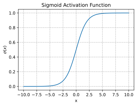
It squashes any real number into the interval \((0, 1)\). The larger the input, the closer the output is to 1; the smaller the input, the closer the output is to 0.
class Sigmoid(Module):"""Elementwise sigmoid activation layer."""def__init__(self):super().__init__()@overridedef forward(self, x: np.ndarray) -> np.ndarray:self.ctx = sigmoid(x)returnself.ctx@overridedef backward(self, grad: np.ndarray) -> np.ndarray:assertself.ctx isnotNone, 'Must call forward before backward.'return grad *self.ctx * (1-self.ctx)
Here, grad is the upstream gradient. In forward, we save self.ctx, namely the sigmoid output \(Y\). This is because backward needs \(Y(1-Y)\) to compute the local derivative.
The problem with sigmoid is also obvious. When the input is very large or very small, the output becomes very close to 1 or 0, and the derivative becomes close to 0:
From the perspective of the Jacobian matrix, this means the diagonal elements become very small. After the upstream gradient is multiplied by such a diagonal Jacobian matrix, it is also reduced. This is the commonly discussed vanishing gradient problem.
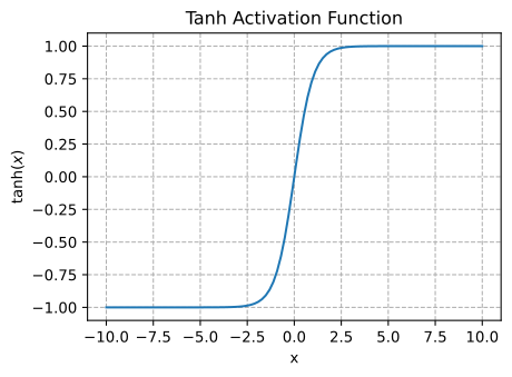
Compared with sigmoid, the output of tanh is centered around 0. That is, it can output both positive and negative values. In many cases, this makes tanh more suitable than sigmoid as a hidden-layer activation function.
The scalar derivative of tanh can also be expressed using the output value. Let:
class Tanh(Module):"""Elementwise hyperbolic tangent activation layer."""def__init__(self):super().__init__()@overridedef forward(self, x: np.ndarray) -> np.ndarray:self.ctx = tanh(x)returnself.ctx@overridedef backward(self, grad: np.ndarray) -> np.ndarray:assertself.ctx isnotNone, 'Must call forward before backward.'return grad * (1- np.square(self.ctx))
However, tanh still has a saturation problem. When the input has a large absolute value, the output approaches 1 or -1, and the local derivative \(1-y^2\) approaches 0. In other words, the diagonal elements of its Jacobian matrix also become very small, so gradients are still easily reduced when passing through this layer.
Therefore, although sigmoid and tanh are historically important, in modern deep learning, ReLU and its variants are more commonly used in hidden layers.
3.2.5 ReLU Activation Function
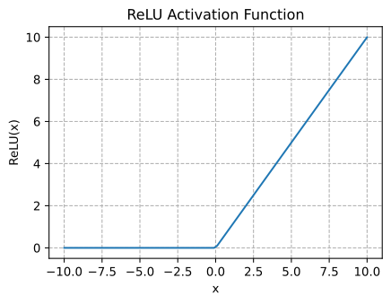
ReLU (Rectified Linear Unit) (Agarap 2026) is one of the most commonly used activation functions today. Its definition is very simple:
\[
\operatorname{ReLU}(x) = \max(0, x)
\]
That is:
\[
\operatorname{ReLU}(x) =
\begin{cases}
x, & x > 0 \\
0, & x \le 0
\end{cases}
\]
The scalar derivative of ReLU is also simple. Let:
\[
y = \operatorname{ReLU}(x)
\]
Then when \(x \ne 0\):
\[
\frac{\partial y}{\partial x} =
\begin{cases}
1, & x > 0 \\
0, & x < 0
\end{cases}
\]
Strictly speaking, ReLU is not differentiable at \(x=0\). In practical implementations, however, we usually directly set the gradient at \(x=0\) to 0. This can be viewed as an implementation convention, and it does not affect the overall training process of neural networks.
This is exactly the same as sigmoid and tanh. Although ReLU is not an invertible function, this does not affect the fact that its Jacobian matrix is diagonal. The reason the off-diagonal entries are 0 is element-wise operation, not function invertibility.
The diagonal elements of the ReLU Jacobian matrix are:
\[
\mathbb{1}(X_{b,d} > 0)
\]
where \(\mathbb{1}(X_{b,d} > 0)\) is the indicator function. It is 1 when \(X_{b,d}>0\), and 0 otherwise. Therefore, backpropagation is:
class ReLU(Module):"""Elementwise rectified linear activation layer."""def__init__(self):super().__init__()@overridedef forward(self, x: np.ndarray) -> np.ndarray:self.ctx = xreturn relu(x)@overridedef backward(self, grad: np.ndarray) -> np.ndarray:assertself.ctx isnotNone, 'Must call forward before backward.'return grad * (self.ctx >0)
Notice that what we save here is the input x, not the output. This is because ReLU’s backward needs to know which positions were greater than 0 during forward propagation.
Of course, we can also save a mask:
class ReLUWithMask(Module):"""Elementwise rectified linear activation layer."""def__init__(self):super().__init__()@overridedef forward(self, x: np.ndarray) -> np.ndarray:self.ctx = x >0return x *self.ctx@overridedef backward(self, grad: np.ndarray) -> np.ndarray:assertself.ctx isnotNone, 'Must call forward before backward.'return grad *self.ctx
These two versions are essentially the same. Neither constructs the full Jacobian matrix; both directly compute the VJP: the upstream gradient multiplied by ReLU’s diagonal Jacobian matrix.
ReLU looks simpler than sigmoid and tanh, but it is very effective in deep networks. One important reason is that when \(x>0\), the local derivative of ReLU is 1:
\[
\operatorname{ReLU}'(x) = 1, \quad x > 0
\]
From the perspective of the Jacobian matrix, this means that at positions where the activation is positive, the diagonal element is 1, so the gradient can pass through this layer relatively directly. It does not quickly shrink due to saturation as it does with sigmoid or tanh.
On the other hand, when \(x \le 0\), the output of ReLU is 0, and the local derivative is also 0. This makes the hidden representation sparse: not every neuron is activated for every sample.
However, ReLU is not without problems. If a neuron stays in the negative half-axis for a long time, the gradient at the corresponding position remains 0, and the parameters may become difficult to update. This is usually called the dead ReLU problem.
Even so, ReLU remains one of the most basic and commonly used activation functions in MLPs, CNNs, and many deep models. In the MLP implementation in this chapter, we will also use ReLU by default.
3.2.6 Activation Functions Usually Do Not Change Tensor Shapes
In neural networks, activation functions usually preserve the shape of their input and output. That is, if a linear layer outputs:
\[
H \in \mathbb{R}^{B \times d}
\]
then after the activation function, we usually still obtain:
\[
A \in \mathbb{R}^{B \times d}
\]
However, we need to distinguish two concepts here:
Whether the shape is preserved;
Whether the operation is element-wise.
For activation functions such as sigmoid, tanh, and ReLU, they both preserve shape and act element-wise. That is:
\[
A_{bj} = \phi(H_{bj})
\]
The output at position \((b,j)\) depends only on the input at position \((b,j)\), and does not depend on any other position. Therefore, if we flatten \(H\) and \(A\) into vectors, the corresponding Jacobian matrix is diagonal:
In this case, \(A_{bj}\) does not depend only on \(H_{bj}\); it also depends on other elements \(H_{bk}\) in the same row. Therefore, although softmax does not change the tensor shape, it is not an element-wise function, and its corresponding Jacobian matrix is not diagonal.
So more accurately:
The reason the backpropagation of element-wise activation functions such as Sigmoid, Tanh, and ReLU can be written as element-wise multiplication is that their Jacobian matrices are diagonal. Whether the shape is preserved is only a surface phenomenon, not the fundamental reason for deciding whether backward can be computed by element-wise multiplication.
3.2.7 Summary
In this section, we first explained the relationship between the Jacobian matrix and backpropagation, then introduced the role of activation functions in MLPs.
For a function from a vector to a vector, the derivative is no longer a scalar, but a Jacobian matrix. Each module in backpropagation is essentially computing:
We introduced sigmoid, tanh, and ReLU. They are all element-wise activation functions, so all off-diagonal elements of their Jacobian matrices are 0. The difference lies in their local derivatives on the diagonal. Sigmoid and tanh squash the input into finite intervals, but when the input has a large absolute value, they easily saturate, making the diagonal elements of the Jacobian matrix close to 0 and causing gradients to shrink. ReLU is simpler: when the input is positive, its local derivative is 1, so it is more commonly used in deep networks. However, when the input stays negative for a long time, the gradient may also remain 0 for a long time, leading to the dead ReLU problem.
In the next section, we will discuss the output layer of classification models. The last layer of an MLP outputs logits, but logits themselves are not probabilities. To train a classification model, we need to combine logits with the true labels to obtain the softmax cross entropy loss and derive its backpropagation.