3.1 From Linear Classifiers to MLPs: Why We Need Hidden Layers

In the previous chapters, we have treated a neural network as a learnable function. Given an input \(x\), the model obtains an output \(\hat{y}\) through a series of computations. Given the true label \(y\), we then use a loss function to measure the gap between the prediction and the label. The process of training a model is essentially the process of repeatedly adjusting its parameters so that this loss becomes smaller.

In this chapter, we start with the classic Multi-Layer Perceptron (MLP) and walk through the basic training process of a neural network from beginning to end. However, the focus of this chapter is not to directly call PyTorch’s nn.Linear, nn.ReLU, and nn.CrossEntropyLoss. Instead, we will first use NumPy to implement the forward and backward propagation of these modules ourselves.

The purpose of doing this is:

First understand what each layer is actually computing by hand, and then return to PyTorch to see what the framework automatically does for us.

In this section, we start from a concrete task: classifying MNIST handwritten digit images. We will first formulate the image classification problem as a linear classifier, then observe the limitations of linear models, and finally naturally introduce hidden layers and activation functions in MLPs.

import numpy as np

rng = np.random.default_rng(seed=42)
print('NumPy version:', np.__version__)

NumPy version: 2.4.6

3.1.1 MNIST Classification Problem

MNIST is a handwritten digit classification dataset. Each image is a grayscale image of size \(28 \times 28\), paired with a digit label:

\[ y \in \{0, 1, 2, \dots, 9\} \]

In other words, this is a 10-class classification problem. After seeing a handwritten digit image, the model needs to determine which class it belongs to.

Figure 3.1.1: MNIST handwritten digit classification dataset (Wikipedia contributors 2026)

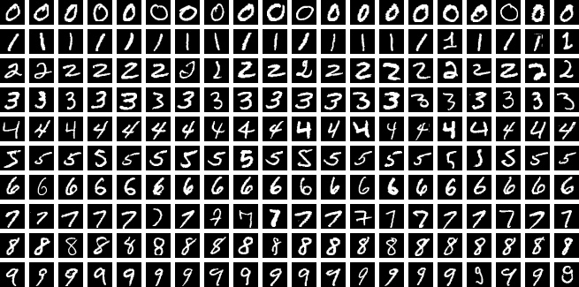
For a computer, a \(28 \times 28\) grayscale image can be viewed as a matrix:

\[ X_{\text{image}} \in \mathbb{R}^{28 \times 28} \]

Each element in the matrix represents the grayscale value of a pixel.

Of course, the most basic MLP is composed of fully connected layers. A fully connected layer usually receives a one-dimensional feature vector, rather than directly receiving a two-dimensional image matrix. This is similar to traditional machine learning classifiers such as support vector machines (SVMs). Therefore, to feed the image into the simplest fully connected model, we usually first flatten the two-dimensional image into a one-dimensional vector:

\[ x \in \mathbb{R}^{28 \times 28} \rightarrow x \in \mathbb{R}^{784} \]

If there are \(B\) images in a batch, then the input can be written as:

\[ X \in \mathbb{R}^{B \times 784} \]

Each row is the flattened vector of one image.

However, this step loses the original two-dimensional spatial structure of the image. For example, after flattening, the model does not directly know which pixels are the top, bottom, left, or right neighbors of a given pixel. When we discuss CNNs and ViTs later, we will revisit how to better make use of image structure. But in an MLP, we first treat the image as an ordinary vector.

batch_size = 4
image_height = 28
image_width = 28

images = rng.random((batch_size, image_height, image_width))
x = images.reshape(batch_size, -1)

print('x.shape:', x.shape)

x.shape: (4, 784)

The output shape is (4, 784). This means each image has been converted from a \(28 \times 28\) matrix into a 784-dimensional vector.

3.1.2 The Simplest Classifier: A Linear Model

After obtaining the input vector, the most direct idea is to use a linear model to map the 784-dimensional input directly to 10 class scores:

\[ Z = XW + b \]

where:

\[ \begin{aligned} X &\in \mathbb{R}^{B \times 784} \\ W &\in \mathbb{R}^{784 \times 10} \\ b &\in \mathbb{R}^{10} \\ Z &\in \mathbb{R}^{B \times 10} \end{aligned} \]

Here, \(Z\) is usually called the logits, which represent the model’s unnormalized scores for each class. For each image, the model outputs 10 numbers, corresponding to its scores for the 10 classes. The higher the score, the more strongly the model tends to believe that the image belongs to that class.

For example, for one image, the model outputs:

\[ z = [z_0, z_1, z_2, \dots, z_9] \]

If \(z_7\) is the largest, we can temporarily regard the model’s prediction as the digit 7:

\[ \hat{y} = \arg\max_j z_j \]

Note that logits are not probabilities yet. They are only unnormalized class scores. Later, we will use softmax to convert logits into probabilities, and then use cross entropy to measure the gap between the prediction and the true label.

First, let us write the forward propagation of this linear classifier in NumPy:

input_dim = 784
num_classes = 10

W = rng.random((input_dim, num_classes))
b = np.zeros(num_classes)
logits = x @ W + b

print('logits.shape:', logits.shape)

logits.shape: (4, 10)

The output shape is (4, 10). This means that for the 4 images in the batch, the model outputs 10 class scores for each image.

3.1.3 What Does a Linear Classifier Learn?

The form of a linear classifier is very simple:

\[ Z = XW + b \]

Figure 3.1.3: Linear classifier model (Zhang et al. 2023, fig. 3.1.2)

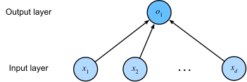
Here, \(X\) is the feature matrix of the input images, \(W\) is the weight matrix, and \(b\) is the bias vector. In the figure above, the input layer is \(X\), the output layer is \(Z\), and the lines in between represent the weight matrix \(W\). At the same time, each output node also has a corresponding bias \(b\), which is not shown in the figure.

If we look at a single class \(j\), its logit is:

\[ z_j = x^\top w_j + b_j \]

where \(w_j\) is the \(j\)-th column of the matrix \(W\). In other words, each class has its own weight vector \(w_j\). The model takes the inner product between the input image \(x\) and this weight vector, then adds the bias \(b_j\), obtaining the score for class \(j\). Intuitively, \(w_j\) can be understood as a template for class \(j\). If the input image matches this template well, the inner product will be larger, and the score for this class will also be higher. When we repeatedly train the model, we are adjusting the \(W\) and \(b\) corresponding to different digits so that they can learn templates that match the corresponding digits, thus making correct classifications on MNIST.

However, the expressive power of this model is limited after all. It can only apply one linear transformation to the input. For a relatively simple dataset like MNIST, a linear classifier can still learn some useful patterns. But if the shape changes in the images are more complex, such as translations, rotations, or variations in stroke width, a purely linear model has a hard time handling all these changes well.

In fact, a linear classifier can only learn decision boundaries of the following form:

\[ x^\top w + b = 0 \]

This is a line, a plane, or a hyperplane in a high-dimensional space. It is suitable for linearly separable data, but it is not enough for more complex nonlinear relationships. This is actually the same as traditional machine learning classifiers such as SVMs: they can only learn linear decision boundaries.

At this point, someone might naturally ask: if one linear layer is not enough, why not just stack several of them?

3.1.4 Is It Useful to Only Stack Linear Layers?

Suppose we connect two linear layers together:

\[ \begin{aligned} H &= XW_1 + b_1 \\ Z &= HW_2 + b_2 \end{aligned} \]

Substituting the first line into the second line gives:

\[ Z = (XW_1 + b_1)W_2 + b_2 \]

After expanding it:

\[ Z = X(W_1W_2) + b_1W_2 + b_2 \]

Let:

\[ \begin{aligned} W' &= W_1W_2 \\ b' &= b_1W_2 + b_2 \end{aligned} \]

Then the entire model becomes:

\[ Z = XW' + b' \]

This is still a linear model. In other words, if there is no nonlinear operation in the middle, stacking multiple linear layers is ultimately still equivalent to a single linear layer. The number of layers increases, but the model’s expressive power does not fundamentally improve.

This is why neural networks cannot be built by stacking only linear layers. We need to insert a nonlinear function between layers, so that the model is no longer just one large purely linear transformation. This nonlinear function is the activation function.

3.1.5 Adding Hidden Layers and Activation Functions

The term activation function comes from biology. A biological neuron receives many input signals. After these signals are weighted and summed, if the stimulus is strong enough, the neuron becomes activated and passes the signal to the next neuron. In artificial neural networks, an activation function simulates this process of a biological neuron being activated. It is a nonlinear function that can apply a nonlinear transformation to its input. In neural networks, an activation function can usually be used as long as it satisfies some basic conditions, such as being nonlinear and differentiable or almost everywhere differentiable.

Now we insert an activation function \(\phi\) between two linear layers:

\[ \begin{aligned} H &= XW_1 + b_1 \\ A &= \phi(H) \\ Z &= AW_2 + b_2 \end{aligned} \]

Here, \(H\) is the hidden layer’s pre-activation, meaning the value before the activation function. \(A\) is the representation after the hidden layer passes through the activation function. \(\phi\) is a nonlinear function, such as sin or cos. Although we will not use them later, they do count as activation functions.

At this point, the model is no longer equivalent to a single linear layer. This is because \(\phi\) applies a nonlinear transformation to the intermediate representation, allowing the model to compose more complex functions.

For MNIST, we can write:

\[ \begin{aligned} X &\in \mathbb{R}^{B \times 784} \\ W_1 &\in \mathbb{R}^{784 \times H} \\ b_1 &\in \mathbb{R}^{H} \\ A &\in \mathbb{R}^{B \times H} \\ W_2 &\in \mathbb{R}^{H \times 10} \\ b_2 &\in \mathbb{R}^{10} \\ Z &\in \mathbb{R}^{B \times 10} \end{aligned} \]

Here, \(H\) is the hidden dimension. For example, we can set \(H=256\), meaning each image is first mapped to a 256-dimensional hidden representation, and then this hidden representation is used to predict the 10 classes. The benefit of doing this is that the model can first extract useful features from the input, namely hidden representations, and then use these features for classification. \(H\) is a hyperparameter, and we can adjust it according to the complexity of the dataset and the expressive power we want the model to have.

In NumPy, this can be written as:

hidden_dim = 256

W1 = rng.random((input_dim, hidden_dim))
b1 = np.zeros(hidden_dim)
W2 = rng.random((hidden_dim, num_classes))
b2 = np.zeros(num_classes)

h = x @ W1 + b1
a = np.maximum(0, h)  # activation function: ReLU
logits = a @ W2 + b2

print('h.shape:', h.shape)
print('a.shape:', a.shape)
print('logits.shape:', logits.shape)

h.shape: (4, 256)
a.shape: (4, 256)
logits.shape: (4, 10)

The activation function we use here is ReLU:

\[ \operatorname{ReLU}(x) = \max(0, x) \]

ReLU turns negative numbers into 0 and keeps positive numbers unchanged. It looks very simple, but it is exactly this nonlinear operation that prevents the composition of two linear transformations from being compressed into one linear transformation. At the same time, it is also one of the most commonly used activation functions in modern neural networks.

3.1.6 Basic Structure of an MLP

The model we now have is the simplest MLP:

\[ X \rightarrow \operatorname{Linear}_1 \rightarrow H_1 \rightarrow \operatorname{ReLU} \rightarrow H_2 \rightarrow \operatorname{Linear}_2 \rightarrow Z \]

Figure 3.1.6: MLP model (Zhang et al. 2023, fig. 4.1.1)

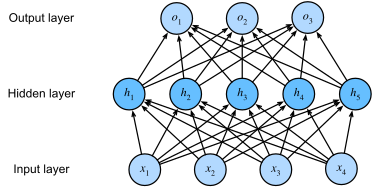
Here, \(\operatorname{Linear}_1\) denotes the first linear layer, \(\operatorname{ReLU}\) is the activation function, \(\operatorname{Linear}_2\) is the second linear layer, \(H_1, H_2\) are the hidden layer’s pre-activation and post-activation representations, and \(Z\) is the output logits.

It can also be written as a function:

\[ f(X) = \operatorname{ReLU}(XW_1 + b_1)W_2 + b_2 \]

There are two points worth noting here.

First, each layer in an MLP usually applies a linear transformation to the last dimension. For MNIST, we flatten each image into a 784-dimensional vector, so the first layer maps 784 dimensions to the hidden dimension \(H\).

Second, our current output \(Z\) is logits, not probabilities yet. Therefore, we need a tool to convert these logits into probabilities and compute the loss. This tool is softmax and cross entropy. Later, we will discuss their forward and backward propagation in detail.

Therefore, the classification pipeline of an MLP can be summarized as:

\[ \text{image} \rightarrow \text{flatten} \rightarrow \text{hidden representation} \rightarrow \text{logits} \rightarrow \text{loss} \]

What we will do in the rest of this chapter is break down each part of this pipeline:

• How do we write the forward and backward propagation of activation functions?
• How do softmax and cross entropy turn logits into a classification loss?
• How do we derive the parameter gradients of a linear layer?
• After multiple modules are connected together, how does the gradient propagate back layer by layer?
• How can we use NumPy to fully train this model on MNIST?

3.1.7 Summary

Starting from the MNIST classification problem, this section introduced the basic idea of moving from a linear classifier to an MLP.

Each MNIST image can be flattened from a \(28 \times 28\) matrix into a 784-dimensional vector. The simplest classifier can use a linear transformation to directly map the input to 10 class logits:

\[ Z = XW + b \]

However, the expressive power of a linear classifier is limited. If we only stack multiple linear layers without inserting nonlinear operations in between, then the entire model is still equivalent to a single linear layer. Therefore, an MLP inserts activation functions between linear layers:

\[ Z = \phi(XW_1 + b_1)W_2 + b_2 \]

Activation functions allow the model to represent more complex nonlinear relationships, and they are an important source of the expressive power of neural networks.

In the next section, we will focus on common activation functions. We will not only look at their forward propagation forms, but also derive how they pass gradients backward during backpropagation.

References

Wikipedia contributors. 2026. MNIST Database — Wikipedia, the Free Encyclopedia. Https://en.wikipedia.org/w/index.php?title=MNIST_database&oldid=1351132851.

Zhang, Aston, Zachary C. Lipton, Mu Li, and Alexander J. Smola. 2023. Dive into Deep Learning. Cambridge University Press. https://D2L.ai.