In the previous section, we saw that Adam combines the ideas of momentum and RMSprop. On the one hand, it maintains a first-moment estimate of the gradient, \(m_t\), to smooth the update direction. On the other hand, it maintains a second-moment estimate of the squared gradient, \(v_t\), to adaptively scale the step size for different parameters.
In Section 4.1, we briefly mentioned the two concepts of L2 regularization and weight decay. At that time, we said that in SGD, they are equivalent. Adding an L2 regularization term to the loss and directly applying weight decay during the parameter update both eventually cause the parameters to decay uniformly. However, when we move to an adaptive optimizer such as Adam, the two start to differ.
We know that L2 regularization is implemented by adding a regularization term to the loss:
after adding L2 regularization, the gradient seen by the optimizer changes from the original \(g_t\) to:
\[
g_t + \lambda\theta_{t-1}
\]
The original \(g_t\) is responsible for reducing the data loss, while the extra \(\lambda\theta_{t-1}\) is responsible for pulling the parameters toward 0.
Weight decay is another perspective. It does not try to add anything to the loss. Instead, it directly specifies that every time we update the parameters, the parameters themselves should decay a little. The most typical form is:
That is, weight decay is a form of optimizer-level regularization. It directly multiplies the parameters by a coefficient smaller than 1 inside the optimizer update rule.
So, we can first understand the relationship between L2 regularization and weight decay as follows:
L2 regularization: add a regularization term to the loss and penalize large parameters by changing the gradient;
Weight decay: directly shrink the parameters proportionally during the optimizer update.
In ordinary SGD, the update formulas of these two methods happen to be equivalent. But in Adam, they are no longer equivalent, because Adam applies first-moment estimation, second-moment estimation, and adaptive scaling to the gradient. As a result, if we mix the L2 regularization term into Adam’s gradient, the regularization term will also enter Adam’s first- and second-moment estimates and be reweighted by Adam’s adaptive scaling mechanism. In this case, weight decay is no longer an independent and uniform parameter decay operation. Instead, it is reweighted by Adam’s adaptive learning rates.
This leads to a question:
When we use an adaptive optimizer such as Adam, can mixing L2 regularization into the gradient still give us the stable and uniform parameter decay effect we want?
The answer from AdamW (Loshchilov and Hutter 2019) is: do not mix L2 regularization into Adam’s gradient statistics. Instead, decouple it from the gradient update.
from collections.abc import Iterablefrom typing import overrideimport dnnlpyimport dnnlpy.optim as doptimport matplotlib.pyplot as pltimport torchimport torch.nn as nnimport torch.nn.functional as Fimport torch.optim as optimfrom torch import Tensordnnlpy.set_matplotlib_format('svg')print('PyTorch version:', torch.__version__)
PyTorch version: 2.14.0+cpu
4.6.1 L2 Loss and Weight Decay: Why Are They Equivalent in SGD?
First, look at the simplest SGD. Without L2 regularization, the update rule is:
\[
\theta_t = \theta_{t-1} - \eta g_t
\]
If we add L2 regularization to the loss, the gradient becomes \(g_t + \lambda\theta_{t-1}\), so the update rule becomes:
Second, perform the normal SGD update along the original gradient \(g_t\).
Therefore, in ordinary SGD, the following two implementations are equivalent:
Add an L2 regularization term to the loss;
Directly apply weight decay during the parameter update.
Because of this equivalence, L2 regularization and weight decay are often mixed together in many contexts. But this equivalence depends on one premise: the optimizer must update parameters directly using the gradient \(g_t\), as SGD does. Once the optimizer applies additional transformations to the gradient, such as maintaining first and second moments and scaling the update by \(\sqrt{\hat{v}_t}\) in Adam, this equivalence is broken.
4.6.2 Why Does This Cause a Problem in Adam?
Adam’s update is not simply:
\[
\theta_t = \theta_{t-1} - \eta g_t
\]
It first puts the gradient into the first and second moments, then uses the second moment to scale the update. If we directly add L2 regularization to the gradient, the gradient actually seen by Adam becomes:
In SGD, \(\lambda\theta\) is merely a term that pulls the parameters toward 0. But in Adam, \(\lambda\theta\) does not only make the parameters decay. It also enters Adam’s first- and second-moment estimates. In other words, the effect of weight decay is changed by Adam’s adaptive scaling mechanism.
For some parameters, if the second moment \(v_t\) is large, the update of that parameter is divided by a larger \(\sqrt{v_t}\), so the effect of weight decay becomes smaller. For other parameters, if the second moment \(v_t\) is small, the effect of weight decay becomes relatively stronger.
As a result, weight decay is no longer a uniform operation that pulls parameters toward 0. Instead, it is reweighted by Adam’s adaptive learning rates. This creates a problem:
We originally wanted weight decay to control parameter magnitude independently, but it has been mixed together with Adam’s gradient scaling mechanism.
The core idea of AdamW is to separate these two things.
4.6.3 AdamW: Decoupling Parameter Decay from the Gradient Update
The W in AdamW comes from weight decay. Its key idea is very direct:
Weight decay should not be mixed into the gradient. It should act directly on the parameters.
That is, AdamW does not add \(\lambda\theta\) to the gradient \(g_t\). Adam’s first and second moments are still updated only from the original gradient \(g_t\):
You can see that this is very similar to the form of weight decay in SGD. The parameters are first multiplied by a decay coefficient, and then Adam’s adaptive gradient update is applied. Therefore, the core of AdamW is not changing Adam’s first or second moment, but changing how weight decay enters the optimizer.
So, AdamW is Adam’s parameter update plus decoupled weight decay. Here, decoupled means that weight decay and the gradient update are separated.
4.6.4 The Difference Between Adam and AdamW
Now we can compare Adam with L2 regularization and AdamW side by side.
Ordinary Adam with L2 regularization is equivalent to first modifying the gradient:
Whether the penalty is first mixed into the gradient and then adaptively scaled by Adam, or directly applied as a uniform decay to the parameters.
This is also why AdamW has a separate W in its name. It emphasizes how weight decay is handled.
4.6.5 PyTorch Implementation of AdamW
Next, we implement a simplified version of AdamW.
class AdamW(dopt.Optimizer):def__init__(self, params: Iterable[Tensor], lr: float=1e-3, betas: tuple[float, float] = (0.9, 0.999), eps: float=1e-8, weight_decay: float=1e-2, ):super().__init__(params)self.lr = lrself.beta1 = betas[0]self.beta2 = betas[1]self.eps = epsself.weight_decay = weight_decayself.step_count =0self.first_moments = [torch.zeros_like(p) for p inself.params]self.second_moments = [torch.zeros_like(p) for p inself.params]@override@torch.no_grad()def step(self):self.step_count +=1for p, m, v inzip(self.params,self.first_moments,self.second_moments, strict=True, ):if p.grad isNone:continue# Decoupled weight decay: directly shrink parameters. grad = p.gradifself.weight_decay >0: p.mul_(1-self.lr *self.weight_decay) m.mul_(self.beta1).add_(grad, alpha=1-self.beta1) v.mul_(self.beta2).addcmul_(grad, grad, value=1-self.beta2) bias_correction1 =1-pow(self.beta1, self.step_count) bias_correction2 =1-pow(self.beta2, self.step_count) m_hat = m / bias_correction1 v_hat = v / bias_correction2# Adam update: use the original gradient statistics. p.addcdiv_(m_hat, v_hat.sqrt() +self.eps, value=-self.lr)
In this code, the key difference between AdamW and Adam is:
p.mul_(1-self.lr *self.weight_decay)
This step directly decays the parameters, instead of adding weight_decay * p to grad. In other words, AdamW’s weight_decay does not participate in the computation of the first and second moments. m and v still come only from the gradient of the current mini-batch.
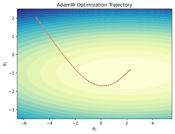
Similarly, we use a simple linear regression task to check whether our AdamW implementation can train normally.
We can see that our AdamW successfully optimizes the parameters from the initial position \((-5.0, 2.0)\) to a position close to the optimum \((2.0, -1.0)\).
In PyTorch, AdamW is used very similarly to Adam:
model = nn.Linear(1, 1)optimizer = optim.AdamW( model.parameters(), lr=1e-3, weight_decay=1e-2,)
The training loop is still the familiar three steps:
x = torch.randn(32, 1)y =2* x +1pred = model(x)loss = F.mse_loss(pred, y)optimizer.zero_grad()loss.backward()optimizer.step()print('Loss:', loss.item())
Loss: 4.001389026641846
4.6.6 Which Parameters Should Use Weight Decay?
In real training, there is one thing we need to pay attention to: not all parameters are suitable for weight decay.
Usually, we apply weight decay to weight matrices, but not necessarily to biases, LayerNorm parameters, or BatchNorm parameters. This is because the main role of weight decay is to limit the complexity of large weight matrices in the model. Biases and the scale and shift parameters in normalization layers do not play exactly the same role as ordinary weight matrices. Directly decaying them may sometimes hurt training.
Therefore, when training Transformers, ViTs, or LLMs, parameters are often divided into two groups:
Parameters that need weight decay;
Parameters that do not need weight decay.
In PyTorch, this can be implemented with parameter groups:
With parameter groups, we can set different weight decay values for different parameters. This prevents parameters that should not be decayed from being affected by weight decay.
4.6.7 Why Is AdamW Commonly Used in Modern Deep Learning?
AdamW is very common in Transformers, ViTs, and many modern deep learning models.
One important reason is that AdamW preserves the advantages of Adam:
It uses first moments to smooth noisy gradients;
It uses second moments to adaptively scale the step size for different parameters;
It is less sensitive to the learning rate, and training is usually relatively stable.
At the same time, AdamW removes weight decay from Adam’s adaptive gradient scaling. As a result, weight decay becomes more like an independent regularization knob. When we tune the learning rate, we mainly affect the gradient update. When we tune weight decay, we mainly affect parameter decay. The roles of the two are easier to understand and easier to tune.
This is also an important reason why AdamW is more suitable than Adam for training modern large models.
Of course, AdamW is not a magic solution. It still requires careful choices of the learning rate, betas, warmup, and scheduler. Especially in models such as Transformers, AdamW is often used together with learning rate warmup, cosine decay, or linear decay.
These topics are more about training practice, and we will discuss them further in a later section on optimizer practice.
4.6.8 Summary
In this section, we started from Adam’s update rule and focused on the relationship between L2 loss and weight decay.
In ordinary SGD, adding L2 regularization to the loss is equivalent to applying weight decay during the parameter update. This is because SGD simply updates parameters along the gradient direction, so \(\lambda\theta\) directly appears as a uniform decay of the parameters.
However, in Adam, if we mix the L2 regularization term into the gradient, the regularization term also enters the first- and second-moment estimates and is reweighted by Adam’s adaptive scaling mechanism. This makes weight decay no longer an independent and uniform parameter decay operation.
The core idea of AdamW is to decouple weight decay. Adam’s first and second moments are updated only from the original gradient, while weight decay acts directly on the parameters. In this way, the learning rate mainly controls the gradient update, and weight decay mainly controls parameter decay, making their meanings clearer.
So far, we have seen a very clear evolution path of optimizers: SGD only looks at the current gradient; momentum remembers the historical direction; Adagrad and RMSprop adjust the effective learning rate of different parameters; Adam combines direction smoothing and adaptive scaling; and AdamW further decouples weight decay in regularization from Adam’s gradient update.
In the next section, we will look at a more modern direction: Muon. It no longer only adjusts the learning rate of each parameter, but further focuses on the update direction of matrix parameters themselves.