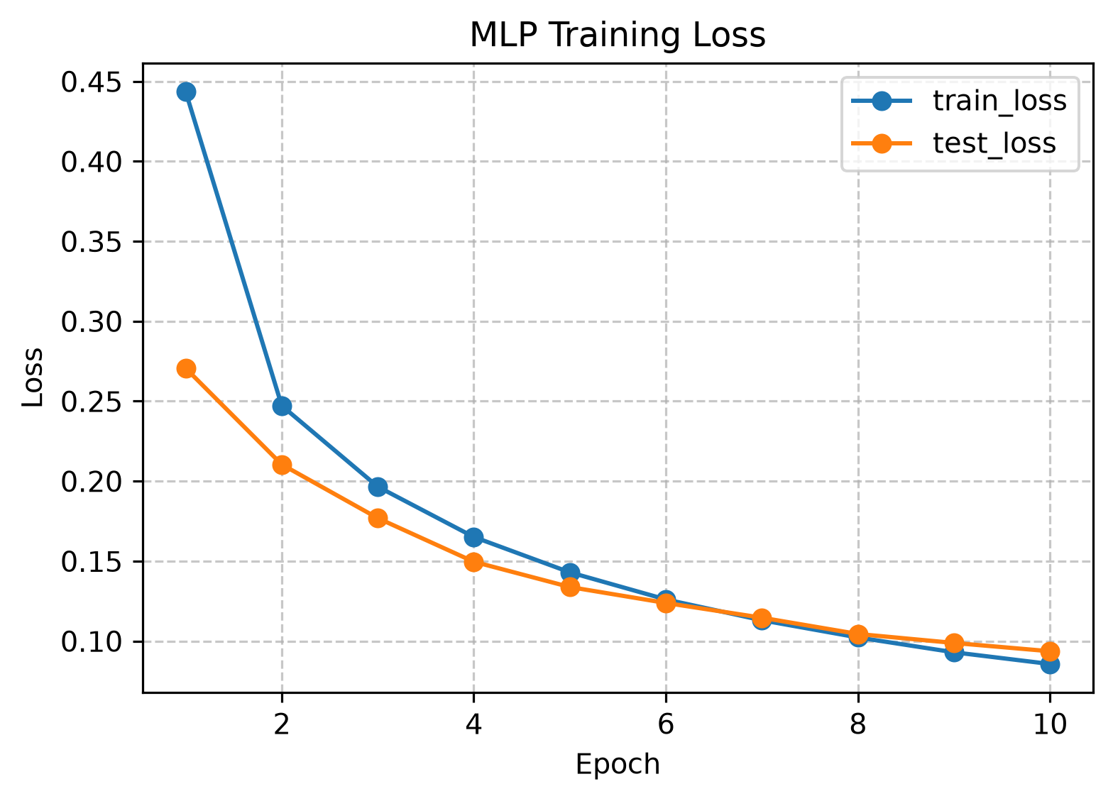
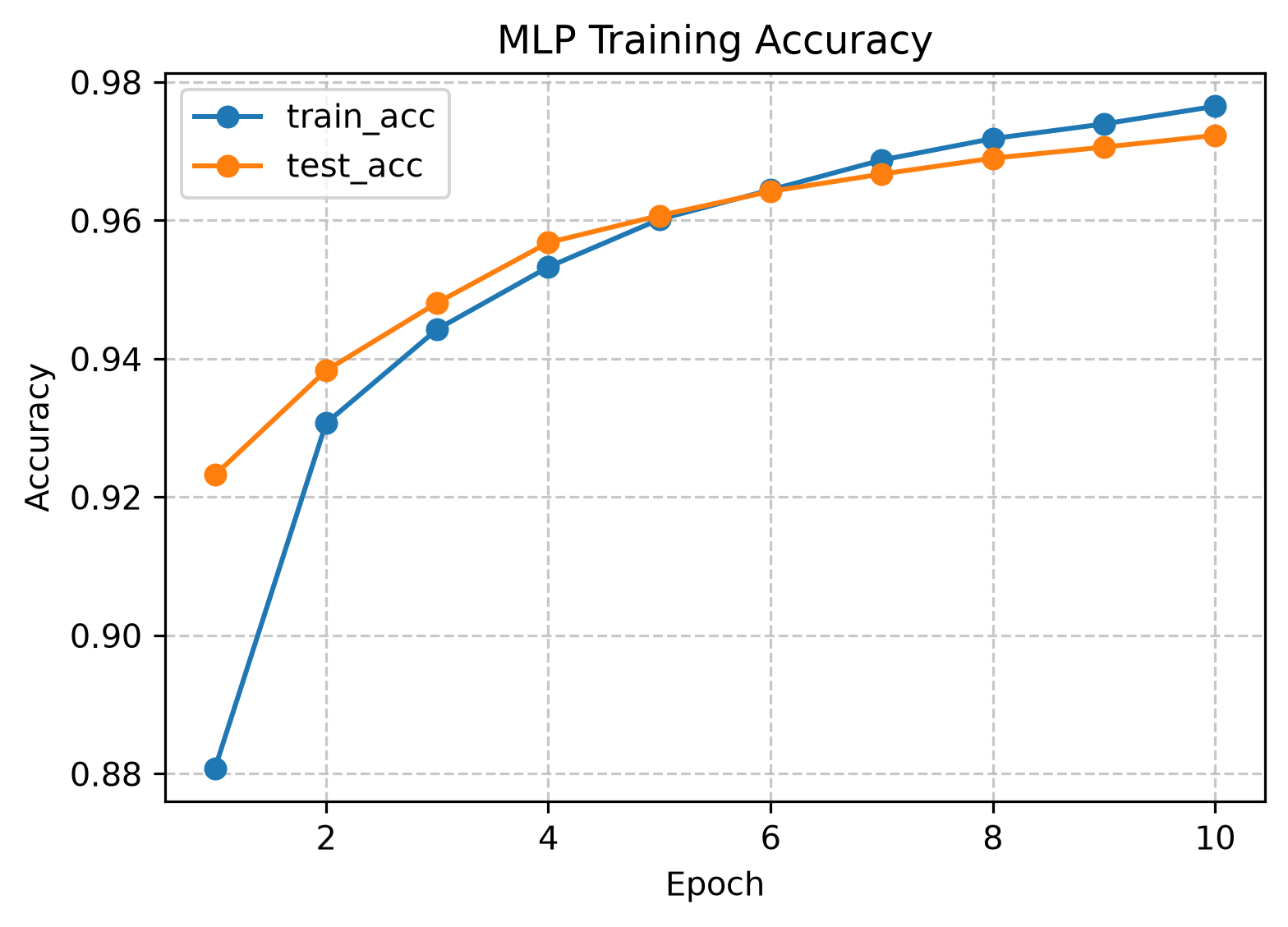
In the previous section, we used NumPy to build a two-layer MLP that can run forward, backward, and update. However, the previous section only used a small randomly generated dataset, which can only check whether the model structure runs correctly. To truly train a neural network, we need to put it on a real dataset and repeatedly perform many parameter updates.
In this section, we train the MLP implemented earlier on the MNIST dataset. To keep the focus on the neural network itself, we still use NumPy to implement the model, loss function, backpropagation, and parameter updates by hand. However, for reading the dataset, we can use the MNIST dataset provided by the torchvision library.
The division of work in this section is:
TorchVision helps us obtain the MNIST data;
NumPy handles the core logic of model training;
PyTorch Autograd is temporarily not involved in the training process.
The complete training process can be written as:
load data -> mini-batch -> forward -> loss -> backward -> update -> evaluate
This is exactly the basic workflow of a supervised learning training loop.
from collections import defaultdictimport mathimport dnnlpyimport dnnlpy.models.mlp as mlpimport matplotlib.pyplot as pltimport numpy as npimport torchvision.datasets as datasetsrng = np.random.default_rng(42)print('Numpy version:', np.__version__)
Numpy version: 2.5.3
3.6.1 Preparing the MNIST Dataset
MNIST is a handwritten digit classification dataset. Each image has size \(28 \times 28\), and the labels range from 0 to 9, giving 10 classes in total.
For an MLP, we temporarily do not treat an image as a two-dimensional grid. Instead, we flatten each image into a vector of length 784:
\[
28 \times 28 = 784
\]
That is, the input shape received by the model is:
The image data read by TorchVision is stored in the data attribute, and the labels are stored in the targets attribute. To train with NumPy later, we convert them into NumPy arrays:
Use reshape(-1, 28 * 28) to flatten each image into a 784-dimensional vector;
Divide by 255.0 to scale pixel values from \([0, 255]\) to \([0, 1]\).
Although this normalization is simple, it is very helpful for training. If the input values are too large, the logits output by the linear layers may also become very large, making training more unstable.
Note that although we flatten the images into vectors, this is only to fit the input format of an MLP. The original images are still two-dimensional; it is just that the MLP does not explicitly use this spatial structure. Later, when we discuss CNNs, we will reintroduce the concept of spatial structure.
3.6.2 Mini-Batch Data Iteration
When training neural networks, we usually do not feed all training data into the model at once. Instead, we split the data into many mini-batches.
If the batch size is \(B\), then one training step only uses:
At the beginning of each epoch, we shuffle the training set. This prevents the model from learning from the samples in exactly the same order in every epoch.
3.6.3 Computing Accuracy
In classification tasks, besides the loss, we often also care about accuracy.
The model outputs logits:
\[
Z \in \mathbb{R}^{B \times 10}
\]
Each row corresponds to the scores of one image over the \(10\) classes. The predicted class is the class with the largest score:
Here we directly use np.argmax to obtain the predicted class, compare it with the true label, and compute the accuracy. Note that although softmax can convert logits into probabilities, it does not change the ranking of logits, so we can directly apply np.argmax to the logits.
3.6.4 Training Loop
Now that we have the mini-batch iterator and evaluation function, together with the model, loss function, and optimizer implemented earlier, we have all the components needed to train a neural network. Next, we can write the complete training loop.
First, prepare the data loaders, model, loss function, and optimizer:
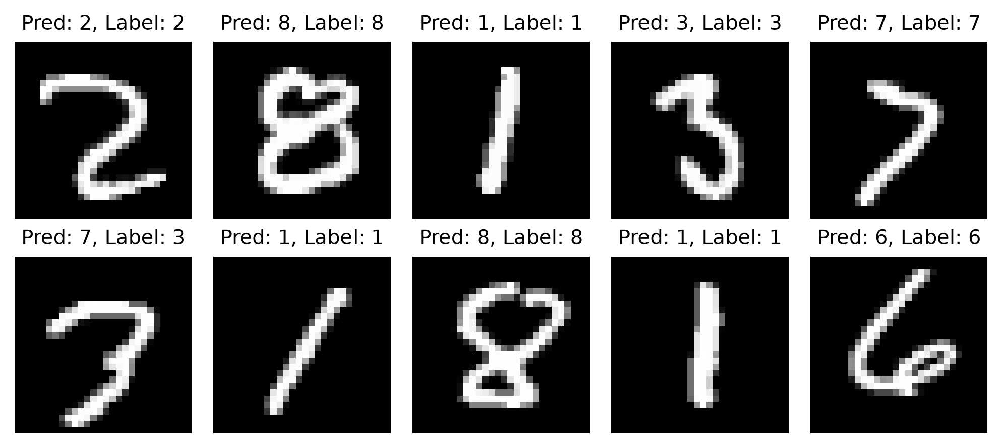
If the prediction is correct, pred and label will be the same. If the prediction is wrong, we can also observe what digit the model confused it with.
This step is not required for training, but it is very useful because it helps us intuitively understand the model’s behavior: which samples it handles well and which samples it handles poorly. From there, we can further analyze the model’s limitations or think about how to improve it.
3.6.7 Limitations of MLPs on Image Tasks
At this point, we have used NumPy to handwrite an MLP that can be trained on MNIST. However, MLPs have an obvious problem when processing images: they directly flatten a \(28 \times 28\) two-dimensional image into a 784-dimensional vector. Although this is simple, it loses the spatial structure in the image.
For example, two neighboring pixels in the original image may still be adjacent after flattening, but the model itself does not know that they come from neighboring positions in a two-dimensional grid. For an MLP, the input is just an ordinary vector:
\[
X = [x_1, x_2, \dots, x_{784}]
\]
It does not explicitly use local regions, translation structure, or two-dimensional neighborhood relationships.
This is why, when processing images later, we usually introduce models that are better suited to image structure, such as convolutional neural networks (CNNs) and Vision Transformers (ViTs). Still, when understanding the training mechanism of neural networks, an MLP remains one of the best starting points, because it already contains the core components of deep learning training:
Learnable parameters;
Forward propagation;
Loss function;
Backpropagation;
Gradient descent updates;
Evaluation on the training set and test set.
3.6.8 Summary
In this section, we put the NumPy MLP implemented earlier onto the MNIST dataset and completed a full training experiment.
We first used torchvision.datasets.MNIST to read the data, then flattened the images into 784-dimensional vectors and normalized them to \([0, 1]\). After that, we handwrote a mini-batch iterator, an accuracy computation function, and a training loop.
This process does not use PyTorch Autograd. All gradients come from the backpropagation formulas we derived and implemented earlier. However, this raises a question:
What if the gradients we computed are wrong?
In the next section, we will discuss a very practical gradient checking method: numerical gradient checking.