import dnnlpy
import matplotlib.pyplot as plt
import torch
import torch.nn.functional as F
from torch import Tensor

dnnlpy.set_matplotlib_format('highdpi')
print('PyTorch version:', torch.__version__)
PyTorch version: 2.14.0+cpu
In the previous section, starting from the limitations of MLPs, we understood why CNNs use local connectivity and weight sharing. Local connectivity makes each output position observe only a small input window, while weight sharing allows the same local detector to be reused across the entire image.
But these descriptions are still only intuitive. When implementing a convolutional layer, we also need to answer a series of very specific questions: How does the kernel slide across the input? Exactly how is each output position calculated? Why does convolution sometimes make an image smaller? How do padding and stride change the output size? When the input contains multiple channels, what shape does a kernel have?
In this section, we will bring these questions together. We will begin with the simplest two-dimensional single-channel convolution, then gradually add padding, stride, batch, and channel dimensions. Finally, we will discuss the seemingly unusual but very important \(1 \times 1\) convolution in modern CNNs.
One point should be clarified in advance: deep learning frameworks usually perform element-wise multiplication directly between the kernel and the input window; they do not flip the kernel first. Strictly speaking, nn.Conv2d therefore implements cross-correlation, rather than the discrete convolution in the mathematical definition. However, in deep learning, the kernel itself is learned through training, and flipping it does not change the expressive power of the model, so this operation is still usually called convolution for short.
import dnnlpy
import matplotlib.pyplot as plt
import torch
import torch.nn.functional as F
from torch import Tensor
dnnlpy.set_matplotlib_format('highdpi')
print('PyTorch version:', torch.__version__)PyTorch version: 2.14.0+cpuFirst consider the simplest case: the input is a single-channel two-dimensional image, and the kernel is also a two-dimensional matrix.
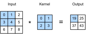
Suppose the input is:
\[ X = \begin{bmatrix} 0 & 1 & 2 \\ 3 & 4 & 5 \\ 6 & 7 & 8 \end{bmatrix} \]
and the kernel is:
\[ K = \begin{bmatrix} 0 & 1 \\ 2 & 3 \end{bmatrix} \]
The kernel first covers the \(2 \times 2\) region in the upper-left corner of the input:
\[ \begin{bmatrix} 0 & 1 \\ 3 & 4 \end{bmatrix} \]
Then we multiply corresponding elements and add them together:
\[ 0 \times 0 + 1 \times 1 + 3 \times 2 + 4 \times 3 = 19 \]
This result is the first element in the upper-left corner of the output. The kernel then moves one position to the right and performs the same calculation on the new local window:
\[ 1 \times 0 + 2 \times 1 + 4 \times 2 + 5 \times 3 = 25 \]
After one row is complete, the kernel moves downward and continues until all valid windows have been processed. The final output is:
\[ Y = \begin{bmatrix} 19 & 25 \\ 37 & 43 \end{bmatrix} \]
For an input with shape \(H \times W\) and a kernel with shape \(K_h \times K_w\), without considering padding or stride for now, the output at position \((i,j)\) can be written as:
\[ Y_{i,j} = \sum_{u=0}^{K_h-1} \sum_{v=0}^{K_w-1} X_{i+u,j+v}K_{u,v} \]
This formula has many indices, but its meaning is simple: take the local window in the input that starts at \((i,j)\), multiply it element by element with the kernel, and add all the results together.
The following implements a minimal version that supports only two-dimensional tensors. It does not yet handle batch, channel, padding, or stride; it is only meant to demonstrate the core sliding-window computation of convolution.
def corr2d(x: Tensor, kernel: Tensor) -> Tensor:
    """Compute 2D cross-correlation for a single-channel input."""
    if x.ndim != 2 or kernel.ndim != 2:
        raise AssertionError('`input` and `kernel` must both be 2D tensors.')

    K_h, K_w = kernel.size()
    h = x.size(0) - K_h + 1
    w = x.size(1) - K_w + 1

    if h <= 0 or w <= 0:
        raise RuntimeError('`kernel` must not be larger than the input.')

    output = x.new_empty(h, w)

    for i in range(h):
        for j in range(w):
            window = x[i : i + K_h, j : j + K_w]
            output[i, j] = torch.sum(window * kernel)

    return output
Let us test it:
x = torch.arange(9, dtype=torch.float32).view(3, 3)
kernel = torch.tensor([[0.0, 1.0], [2.0, 3.0]])

y = corr2d(x, kernel)

print('Input:', x, sep='\n')
print('Kernel:', kernel, sep='\n')
print('Output:', y, sep='\n')
Input:
tensor([[0., 1., 2.],
[3., 4., 5.],
[6., 7., 8.]])
Kernel:
tensor([[0., 1.],
[2., 3.]])
Output:
tensor([[19., 25.],
[37., 43.]])This implementation already captures the two most important ideas in convolution:
Padding, stride, and multi-channel convolution later do not change this core. They only determine how the window moves and which dimensions are included in each window.
A kernel does not have a fixed meaning. It is simply a set of learnable parameters, and different parameters respond to different local patterns.
For example, the following kernel compares pixels on the left and right sides of a local region:
\[ K_{\text{vertical}} = \begin{bmatrix} -1 & 0 & 1 \\ -1 & 0 & 1 \\ -1 & 0 & 1 \end{bmatrix} \]
If the pixels on the left side of a window are darker and those on the right are brighter, the convolution result will be relatively large. Thus, this kernel can detect a vertical change in brightness. Similarly, reversing the direction of the kernel allows it to detect horizontal edges.
image = torch.zeros(10, 10)
image[:, 5:] = 1.0

kernel = torch.tensor(
    [
        [-1.0, 0.0, 1.0],
        [-1.0, 0.0, 1.0],
        [-1.0, 0.0, 1.0],
    ]
)
response = corr2d(image, kernel)

fig = plt.figure(1, figsize=(6, 3))
ax1 = fig.add_subplot(1, 2, 1)
ax1.imshow(image, cmap='gray', vmin=0, vmax=1)
ax1.set_xticks([])
ax1.set_yticks([])
ax1.set_title('Input')
ax2 = fig.add_subplot(1, 2, 2)
ax2.imshow(response, cmap='gray')
ax2.set_xticks([])
ax2.set_yticks([])
ax2.set_title('Vertical Edge Response')
plt.show()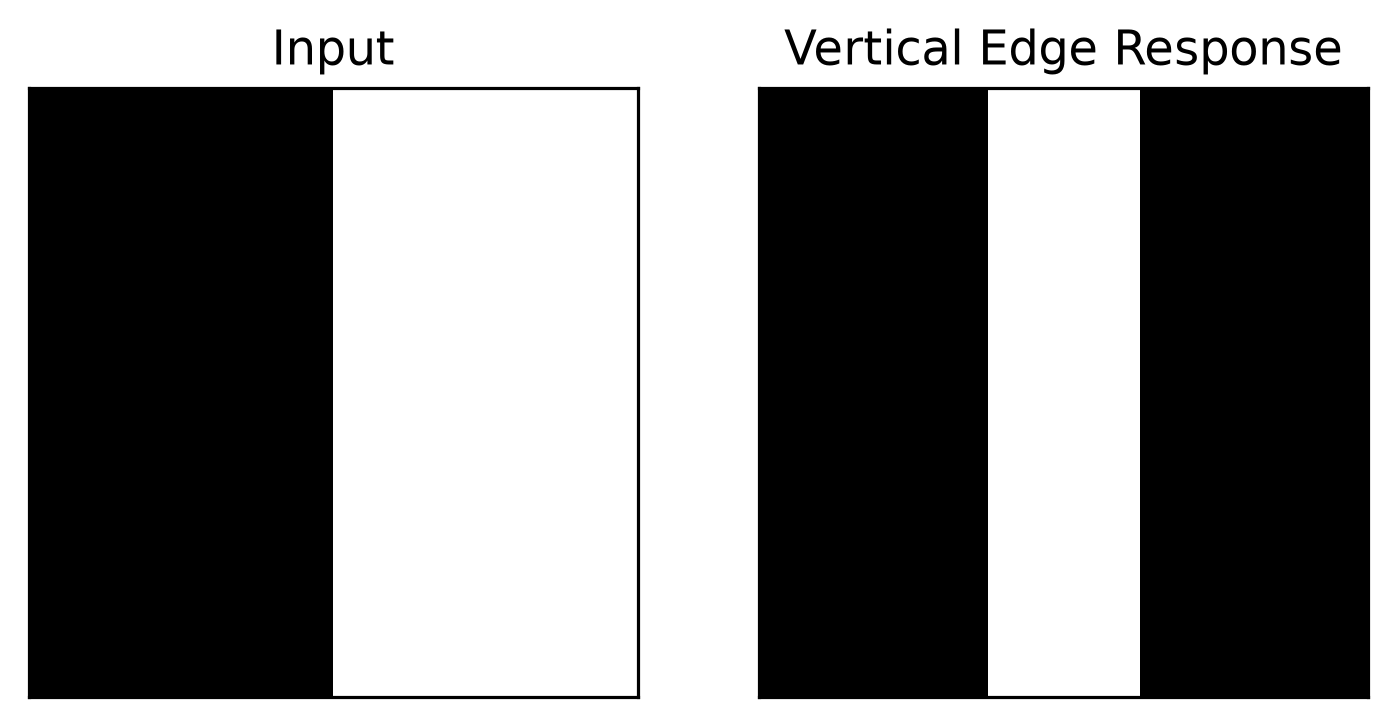
Here, we specified the kernel by hand. In a real CNN, kernels are usually learned automatically through backpropagation, just like the weights of a linear layer. Shallow convolutional kernels may gradually learn to respond to edges, color changes, and simple textures, while deeper kernels combine features extracted earlier to form more complex visual representations.
Thus, a convolutional layer does not prescribe which patterns the network should detect in advance. Instead, it constrains how patterns are detected: each computation sees only a local window, and the same set of parameters is shared across all positions.
If the kernel can be placed only at positions completely inside the input, the spatial dimensions usually become smaller after convolution.
For example, if a \(5 \times 5\) input uses a \(3 \times 3\) kernel, the kernel can move to only 3 valid positions in both the height and width directions, so the output size is \(3 \times 3\). If convolution is repeated, the spatial dimensions continue to shrink:
\[ 5 \times 5 \xrightarrow{3 \times 3} 3 \times 3 \xrightarrow{3 \times 3} 1 \times 1 \]
This also creates another problem: boundary pixels participate in the computation fewer times than center pixels. A center pixel appears in multiple local windows, while a corner pixel may be used only once.
Padding adds extra pixels around the input boundary. The most common choice is to add zeros, which is called zero padding. For a two-dimensional input, if \(P_h\) rows are added above and below in the height direction, and \(P_w\) columns are added to the left and right in the width direction, the original input size \(H\times W\) becomes:
\[ (H + 2 P_h) \times (W + 2 P_w) \]
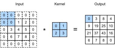
Let us observe what happens when a \(3 \times 3\) input is surrounded by one layer of zero padding.
x = torch.arange(1, 10, dtype=torch.float32)
x = x.view(1, 1, 3, 3)
padded = F.pad(x, pad=(1, 1, 1, 1))

print('Original input:', x[0, 0], sep='\n')
print('After padding=1:', padded[0, 0], sep='\n')
Original input:
tensor([[1., 2., 3.],
[4., 5., 6.],
[7., 8., 9.]])
After padding=1:
tensor([[0., 0., 0., 0., 0.],
[0., 1., 2., 3., 0.],
[0., 4., 5., 6., 0.],
[0., 7., 8., 9., 0.],
[0., 0., 0., 0., 0.]])In PyTorch, the order for two-dimensional padding is:
(left, right, top, bottom)For an odd-sized kernel, if the stride is 1 and the padding on each side is:
\[ P_h=\frac{K_h-1}{2}, \qquad P_w=\frac{K_w-1}{2} \]
then the height and width of the image remain unchanged before and after convolution. For example, a \(3\times 3\) kernel uses padding=1, and a \(5\times 5\) kernel uses padding=2.
This way of preserving the spatial dimensions is often called same padding. In contrast, valid padding does not add any pixels, so the spatial dimensions become smaller after convolution. However, note that strict same padding also depends on the stride and whether the kernel has an even size. When the stride is greater than 1, the output dimensions usually still decrease.
The kernel in the previous examples moved only one pixel at a time, corresponding to stride=1. But a kernel can also move multiple positions at once. For example, when the stride is 2, the kernel skips two pixels at a time in both the horizontal and vertical directions. This produces fewer output positions and causes the spatial dimensions to decrease more quickly.
Stride does not change the computation inside each local window. It changes only the position of the window’s starting point. When the stride is not 1, the input window corresponding to output position \((i,j)\) no longer starts at \((i,j)\), but at:
\[ (i S_h, j S_w) \]
where \(S_h\) and \(S_w\) are the strides in the height and width directions, respectively.
Therefore, a single-channel convolution with stride can be written as:
\[ Y_{i,j} = \sum_{u=0}^{K_h-1} \sum_{v=0}^{K_w-1} X_{iS_h+u,jS_w+v}K_{u,v} \]
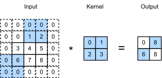
The following uses the same input and kernel to compare the outputs for strides of 1 and 2.
x = torch.arange(1, 26, dtype=torch.float32).view(1, 1, 5, 5)
kernel = torch.ones(1, 1, 3, 3)

stride1 = F.conv2d(x, kernel, stride=1)
stride2 = F.conv2d(x, kernel, stride=2)

print('Input shape:', x.shape)
print('Output shape with stride=1:', stride1.shape)
print('Output shape with stride=2:', stride2.shape)
print('Output with stride=1:', stride1[0, 0], sep='\n')
print('Output with stride=2:', stride2[0, 0], sep='\n')
Input shape: torch.Size([1, 1, 5, 5])
Output shape with stride=1: torch.Size([1, 1, 3, 3])
Output shape with stride=2: torch.Size([1, 1, 2, 2])
Output with stride=1:
tensor([[ 63., 72., 81.],
[108., 117., 126.],
[153., 162., 171.]])
Output with stride=2:
tensor([[ 63., 81.],
[153., 171.]])A convolution with a stride greater than one performs two tasks at once:
Therefore, modern CNNs often use strided convolution in place of some pooling layers. However, a larger stride also means that fewer spatial positions are retained in the output, so downsampling too early may lose details.
We can now combine kernel, padding, and stride to derive the output size of a convolution.
First consider the height direction. If the original input height is \(H\), its effective height after padding above and below is:
\[ H + 2 P_h \]
The kernel height is \(K_h\). The first window starts at position 0, and the starting point of the last valid window is at most:
\[ H + 2 P_h - K_h \]
Since adjacent window starting points are \(S_h\) apart, the output height is:
\[ H_{\text{out}} = \left\lfloor \frac{H+2P_h-K_h}{S_h} \right\rfloor+1 \]
The width direction is analogous:
\[ W_{\text{out}} = \left\lfloor \frac{W+2P_w-K_w}{S_w} \right\rfloor+1 \]
For example, if the input size is \(32\times 32\), the kernel is \(3\times 3\), the padding is 1, and the stride is 1, then:
\[ H_{\text{out}} = \left\lfloor \frac{32+2-3}{1} \right\rfloor + 1 = 32 \]
If the stride is changed to 2:
\[ H_{\text{out}} = \left\lfloor \frac{32+2-3}{2} \right\rfloor + 1 = 16 \]
The following defines a small function and compares it with the actual output of F.conv2d.
def conv2d_output_size(
    input_size: int, kernel_size: int, stride: int = 1, padding: int = 0
) -> int:
    return (input_size + 2 * padding - kernel_size) // stride + 1


x = torch.randn(1, 1, 32, 32)
weight = torch.randn(1, 1, 3, 3)

for stride, padding in [(1, 0), (1, 1), (2, 1)]:
    actual = conv2d_output_size(
        input_size=32,
        kernel_size=3,
        stride=stride,
        padding=padding,
    )
    expected = F.conv2d(x, weight, stride=stride, padding=padding)

    print(
        f'stride={stride}, padding={padding}: '
        f'actual={actual}, expected={expected.size(-1)}'
    )
stride=1, padding=0: actual=30, expected=30
stride=1, padding=1: actual=32, expected=32
stride=2, padding=1: actual=16, expected=16The output-size formula is one of the most commonly used formulas for understanding CNN architectures. When reading a network diagram, as long as you know the input size, kernel, padding, and stride, you can calculate the feature-map size layer by layer.
Note that we have not included dilation for now. Dilated convolution spreads out the sampling points inside a kernel, which is equivalent to increasing the kernel’s effective size. We will discuss it later when it is actually needed.
Here is a classic visualization project for CNN convolution operations: Convolution Arithmetic. Through a series of animations, it intuitively shows how kernels slide across input feature maps, covering ordinary convolution, different strides and padding schemes, dilated convolution, transposed convolution, and other operations.
So far, both the input and the kernel have been two-dimensional. In practice, images usually also contain a channel dimension.
For example, an RGB image can be written as:
\[ X\in\mathbb{R}^{3\times H\times W} \]
The three channels contain the pixel values for red, green, and blue. In this case, a kernel cannot process only one of the channels, because it would be unable to use information from the different colors at the same time.
Therefore, for a feature map with \(C_{\text{in}}\) input channels, a complete kernel must also contain \(C_{\text{in}}\) channels:
\[ K\in\mathbb{R}^{C_{\text{in}}\times K_h\times K_w} \]
When calculating a particular output position, each input channel performs a local multiply-and-add with its corresponding kernel slice, and the results are then summed along the channel dimension. For a single output channel:
\[ Y_{i,j} = \sum_{c=0}^{C_{\text{in}}-1} \sum_{u=0}^{K_h-1} \sum_{v=0}^{K_w-1} X_{c,i+u,j+v}K_{c,u,v} \]
In other words, multiple input channels do not independently produce multiple final outputs. Their information is first combined into a single output feature map.
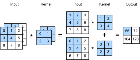
The following constructs a two-channel input and manually verifies one multi-channel convolution.
x = torch.tensor(
    [
        [[1.0, 2.0, 3.0], [4.0, 5.0, 6.0], [7.0, 8.0, 9.0]],
        [[9.0, 8.0, 7.0], [6.0, 5.0, 4.0], [3.0, 2.0, 1.0]],
    ]
)
kernel = torch.tensor(
    [
        [[1.0, 0.0], [0.0, 1.0]],
        [[0.0, 1.0], [1.0, 0.0]],
    ]
)

actual = sum(corr2d(x[c], kernel[c]) for c in range(x.size(0)))
expected = F.conv2d(x.unsqueeze(0), kernel.unsqueeze(0))
flag = torch.allclose(actual, expected[0, 0])

print('Manual output:', actual, sep='\n')
print('PyTorch output:', expected[0, 0], sep='\n')
print('Is manual output equal to PyTorch output?', flag)
Manual output:
tensor([[20., 20.],
[20., 20.]])
PyTorch output:
tensor([[20., 20.],
[20., 20.]])
Is manual output equal to PyTorch output? TrueHere, the shape of x is (2, 3, 3), representing 2 input channels; the shape of kernel is (2, 2, 2), meaning that this kernel also contains 2 input channels. The two channels are computed separately and then added, producing only 1 output channel in the end.
A single kernel can produce only one output feature map. If the network should detect multiple types of local patterns at the same time, it needs multiple different kernels.
For example, one kernel may respond more strongly to vertical edges, another may respond to horizontal edges, and others may learn color changes or textures. Each kernel produces one output channel. Stacking these results produces a multi-channel output.
If the number of input channels is \(C_{\text{in}}\) and the number of output channels is \(C_{\text{out}}\), the shape of the convolutional layer’s weights is:
\[ W \in \mathbb{R}^{C_{\text{out}}\times C_{\text{in}}\times K_h\times K_w} \]
This is also the dimension order used by PyTorch Conv2d weights:
(out_channels, in_channels, kernel_height, kernel_width)If bias is enabled, each output channel also has an independent bias, so:
\[ b \in \mathbb{R}^{C_{\text{out}}} \]
For an input with a batch dimension, the complete shape is:
\[ X \in \mathbb{R}^{N\times C_{\text{in}}\times H\times W} \]
The output shape is:
\[ Y \in \mathbb{R}^{N\times C_{\text{out}}\times H_{\text{out}}\times W_{\text{out}}} \]
Here, \(N\) is the batch size. The convolutional layer uses the same set of weights for every sample in the batch, but different samples are not mixed with one another.
x = torch.randn(4, 3, 32, 32)
weight = torch.randn(16, 3, 3, 3)
bias = torch.randn(16)

y = F.conv2d(x, weight, bias=bias, stride=1, padding=1)

print('Input shape:', x.shape)
print('Weight shape:', weight.shape)
print('Bias shape:', bias.shape)
print('Output shape:', y.shape)
Input shape: torch.Size([4, 3, 32, 32])
Weight shape: torch.Size([16, 3, 3, 3])
Bias shape: torch.Size([16])
Output shape: torch.Size([4, 16, 32, 32])In this example:
Therefore, the output shape is (4, 16, 32, 32).
The number of parameters in a convolutional layer can also be obtained directly from the weight shape:
\[ C_{\text{out}}C_{\text{in}}K_hK_w + C_{\text{out}} \]
Unlike a fully connected layer, this parameter count does not depend on the height and width of the input image. As long as the number of input channels remains the same, the same convolutional layer can process both \(32\times 32\) images and larger spatial dimensions.
The \(1\times 1\) convolution may seem strange the first time you encounter it. Its spatial window contains only one position, so it cannot observe neighboring pixels or directly detect edges. Why is it still useful?
The key point is:
Although the spatial size of the kernel is \(1\times 1\), it still covers all input channels.
Suppose the channel vector at a particular input position is:
\[ x_{i,j}\in\mathbb{R}^{C_{\text{in}}} \]
A \(1\times 1\) convolution with \(C_{\text{out}}\) output channels performs the same linear transformation at every spatial position:
\[ y_{i,j} = Wx_{i,j} + b \]
where:
\[ W\in\mathbb{R}^{C_{\text{out}}\times C_{\text{in}}} \]
Thus, the main purpose of a \(1\times 1\) convolution is not to mix a spatial neighborhood but to mix channel information. It can:
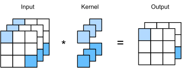
Moreover, a \(1\times 1\) convolution is equivalent to a linear layer applied independently at each spatial position. As long as we treat the channel dimension of the input tensor as the feature dimension, a \(1\times 1\) convolution applies the same linear transformation at every spatial position.
The following verifies the equivalence between a \(1\times 1\) convolution and a position-wise linear layer.
x = torch.randn(2, 3, 4, 5)
weight = torch.randn(6, 3, 1, 1)
bias = torch.randn(6)

conv_output = F.conv2d(x, weight, bias=bias)

x = x.permute(0, 2, 3, 1)
linear_weight = weight[:, :, 0, 0]
linear_output = F.linear(x, linear_weight, bias)
linear_output = linear_output.permute(0, 3, 1, 2)

print('Conv output shape:', conv_output.shape)
print('Linear output shape:', linear_output.shape)

flag = torch.allclose(conv_output, linear_output, atol=1e-6)
print('Is Conv2d output equal to Linear output?', flag)
Conv output shape: torch.Size([2, 6, 4, 5])
Linear output shape: torch.Size([2, 6, 4, 5])
Is Conv2d output equal to Linear output? TrueThe two computations are exactly the same. The only difference is that Conv2d naturally applies this linear transformation to every spatial position while preserving the (N, C, H, W) image layout.
\(1\times 1\) convolutions appear repeatedly later in GoogLeNet, SqueezeNet, MobileNet, and ResNet. For now, remember their most important meaning:
An ordinary spatial convolution mixes both spatial and channel information, while a \(1\times 1\) convolution mixes channels only at each position.
Starting from the simplest single-channel two-dimensional convolution, this section gradually filled in the most important computation rules used by a practical Conv2d.
The core of a convolutional layer remains a local window and weight sharing. The kernel slides across the input, and each output position is computed from a local window and the same set of weights. Padding adds elements around the input boundary to control boundary information and output size; stride determines the kernel’s step size and the downsampling rate of the feature map.
For a multi-channel input, a kernel must cover all input channels and sum along the channel dimension. Multiple different kernels produce multiple output channels, so the weight shape of Conv2d is:
\[ (C_{\text{out}}, C_{\text{in}}, K_h, K_w) \]
Although a \(1\times 1\) convolution does not aggregate neighboring spatial positions, it can mix channels at every position and flexibly increase or decrease the number of channels.
At this point, we know how a convolutional layer should be computed, but this section relied mainly on F.conv2d to perform the actual operations involving batch, channel, padding, and stride. In the next section, we will combine these rules to implement a more complete Conv2d from scratch, and then compare its parameters, initialization, and outputs with nn.Conv2d.