11.1 From CNN to Vision Transformer: Treating Images as Sequences

In the previous chapters, we have seen how Transformer processes sequences. Whether it is the Encoder-Decoder Transformer used in machine translation, or models that use only the encoder or only the decoder, their input is essentially a token sequence:
\[ X = [x_1, x_2, \dots, x_n] \]
If the input is a sequence, this is very natural. A sentence is already word after word, code is already symbol after symbol, and speech can also be unfolded over time into an audio sequence. So the model only needs to map each token into a vector, and then pass it to self-attention for processing.
But images are different. An image is usually a three-dimensional tensor:
\[ X \in \mathbb{R}^{C \times H \times W} \]
where \(C\) is the number of channels, and \(H\) and \(W\) are the height and width of the image. It does not look like a sequence of tokens, but rather like a two-dimensional spatial structure. Each pixel has both a value and a spatial position; neighboring pixels are usually highly correlated, and objects are often gradually composed from local textures, edges, and parts.
So, if we want to apply Transformer to images, the first problem we face is:
Transformer can only process token sequences, but an image is not a sequence. What should we do?
Vision Transformer, abbreviated as ViT (Dosovitskiy et al. 2021), starts exactly from this problem. Its idea is actually very simple: since Transformer is good at processing token sequences, why don’t we cut an image into a group of small blocks, treat each small block as a token, and then use Transformer to model the relationships among these image tokens?
In this section, we will not rush to write the complete ViT architecture. Instead, we first understand why it is designed this way. In other words, we will start from how CNN models images, and gradually arrive at the basic idea of ViT: treating images as sequences.
11.1.1 Why Images Have Long Been Suitable for CNNs
Before ViT appeared, Convolutional Neural Networks (CNNs) had long been the mainstream architecture in vision tasks. The reason CNNs are suitable for images is not accidental. It is because their structure builds in several assumptions that match image properties very well.
The first assumption is locality. A pixel in an image is usually closely related to the pixels around it, rather than to pixels far away. For example, edges, textures, and corners can often be recognized from local regions. Therefore, CNNs use small convolution kernels, such as \(3 \times 3\) or \(5 \times 5\), to extract features from local regions first.
The second assumption is translation equivariance. In a CNN, the same convolution kernel slides across the whole image. That is, the model uses the same set of parameters to detect similar patterns at different positions. If a convolution kernel has learned to detect vertical edges, then it can detect vertical edges not only in the upper-left corner, but also in the lower-right corner. This matches an intuition in image tasks: the same visual pattern may appear at different positions in an image. This is also the parameter-sharing mechanism of CNNs.
The third assumption is hierarchical structure. Shallow convolution layers usually learn low-level features such as edges, colors, and textures; deeper layers gradually combine these low-level features to form representations of parts, objects, or even scenes. As the network becomes deeper, the receptive field of each position gradually expands, and the model can integrate global semantics from local information step by step. For example, in an image of a cat, pixels near the cat’s ears form local edges and textures; local regions near the cat’s face form structures such as eyes, nose, and whiskers; multiple local structures are then combined to form the overall concept of “cat.”
Therefore, the way CNNs look at images can roughly be understood as:
Look locally first, then gradually expand the field of view through layer-by-layer stacking.
This design is very suitable for images and also very efficient. A convolution layer does not need to let every position interact with every other position from the beginning. Instead, it first focuses on nearby regions, and then propagates information gradually through multiple layers. Many classic vision models, such as AlexNet, VGG, and ResNet, are built on this idea.
However, this also brings up a natural question: if two regions in an image are far apart, but they are highly related semantically, CNNs need many layers before they can fully exchange information. Then, is there a structure that allows any two regions in an image to interact directly from the beginning?
This is exactly what self-attention is good at.
11.1.2 Self-Attention: Another Way to Model Images
In Transformer, the core role of self-attention is to let each token in a sequence retrieve information from other tokens according to the current need. For a sequence of length \(n\), each token can theoretically attend directly to any other token in the sequence.
If we move this idea to images, we get a very appealing thought: each region in an image does not necessarily have to expand its receptive field layer by layer through local convolution first. It can also directly establish relationships with other regions.
For example, in an animal image, the head, body, and tail may be far apart. CNNs usually need multiple convolution layers to gradually integrate the information of these parts. But if we use self-attention, the image token representing the head can directly attend to the token representing the body or the tail. The model does not have to wait until many layers later to obtain global information; instead, global information exchange can happen in every layer.
Of course, this brings us back to the problem at the very beginning:
The input of self-attention is a token sequence, but an image is not already a token sequence.
If we want images to enter Transformer, we must first figure out one thing: what exactly are the tokens in an image?
Some people may say that a token is the most basic unit of a sentence, and a pixel is the basic unit of an image. Then can’t we just treat each pixel as a token?
The idea is good. But if we do that, a \(224 \times 224\) image becomes \(224 \times 224 = 50176\) tokens. We know that self-attention needs to compute relationships between all pairs of tokens, and the attention matrix grows quadratically with the number of tokens. If there are 50176 tokens, the attention matrix will be extremely large, and both computation and GPU memory cost will be hard to afford. Taking float32 as an example, this attention matrix alone requires about 10 GB of memory. And this is only one attention matrix, not to mention that we still need to stack multiple layers.
So ViT does not treat a single pixel as a token. It uses a compromise: cut the image into a group of small blocks, usually square ones. Each small block is called a patch, and each patch is treated as a token.
This step is critical. It turns an image from a two-dimensional grid into a token sequence, without making the number of tokens too large, and it allows Transformer to take over the subsequent modeling directly.
11.1.3 Cutting an Image into Patches
Suppose we have an image:
\[ X \in \mathbb{R}^{C \times H \times W} \]
Assume the patch size is \(P\), meaning each patch has size \(P \times P\). If both \(H\) and \(W\) are divisible by \(P\), then the whole image can be cut into
\[ N = \frac{H}{P} \times \frac{W}{P} \]
patches.
For example, for a \(224 \times 224\) RGB image, if we use \(16 \times 16\) patches, the number of patches is:
\[ N = \frac{224}{16} \times \frac{224}{16} = 14 \times 14 = 196 \]
In this way, an image that originally has 50176 pixel positions is converted into 196 patch tokens. This sequence length is much more reasonable for Transformer.
At this point, each patch itself is still a small image block. For an RGB image, the shape of one patch is:
\[ (C, P, P) \]
If we flatten it into a vector, we get:
\[ x_i \in \mathbb{R}^{C \times P^2} \]
Thus, an image can be represented as a group of patch vectors:
\[ \text{image} \rightarrow [x_1, x_2, \dots, x_N] \]
Now the image has finally become a sequence. It is just that the tokens in this sequence are not words, but image patches.
Intuitively, ViT does something simple but crucial:
Treat local regions in an image as visual tokens.
In this way, Transformer is no longer limited to language sequences. As long as we can split the input into a group of tokens, it can use self-attention to model the relationships among them. The patch embedding, class token, positional embedding, and ViT Encoder that we will discuss in the following sections all revolve around this sentence.
11.1.4 How Are Patch Sequences Different from Word Sequences?
Although ViT turns an image into a token sequence, an image patch sequence is not exactly the same as a natural-language word sequence.
In language, token order usually has a strong one-dimensional structure. The order before and after a word directly affects the meaning of a sentence. For example, “dog bites man” and “man bites dog” contain the same words, but their order is different, so their meanings are different.
Images also have positional structure, but it is originally two-dimensional. A patch has not only previous-next relationships, but also up-down-left-right relationships. After a two-dimensional patch grid is flattened into a one-dimensional sequence, the original spatial structure is weakened. For example, the upper-left patch and the lower-right patch are just two positions in the sequence; without additional information, the model does not know their specific spatial relationship in the original image.
This brings up a new problem:
If the image is flattened into a sequence, does the model still know where each patch originally was?
The answer is: patch content alone is not enough. Even if two patches have the same content, if one comes from the upper-left corner and the other from the lower-right corner, they may play different roles in visual semantics. Therefore, ViT later needs to add positional encoding to bring back the spatial position information of the patches.
However, before entering positional encoding, we still need to solve another problem: the flattened patch vector is only an arrangement of raw pixels. It is not yet the token embedding actually used by Transformer.
In NLP, a token ID first passes through an embedding layer and becomes a fixed-dimensional vector. Similarly, after an image patch is flattened, it also needs to pass through a learnable linear projection and become the patch embedding used by Transformer.
Why do we need this? Because flattening only rearranges pixels into a vector. It has no learning ability by itself. For example, after a \((3, 16, 16)\) patch is flattened, we get a 768-dimensional vector, but this vector is only an arrangement of raw pixel values and has not gone through any feature transformation. So we need to project it into a feature space, allowing the model to better capture semantic relationships among patches rather than being limited by the arrangement of raw pixel values.
Overall, the input construction of ViT roughly contains three steps:
- Cut the image into patches and flatten each patch into a vector;
- Project each patch vector to the hidden dimension of Transformer to obtain a patch embedding;
- Add positional encoding to each patch embedding so that the model knows where it comes from in the image.
These are the topics we will discuss in detail in the next few sections.
11.1.5 The Overall Idea of ViT
Now we can first look at the overall structure of ViT. It does not reinvent a completely different Transformer for images, but instead reuses the standard Transformer Encoder as much as possible. The truly important change happens at the input side: ViT first converts the image into a patch token sequence.
The overall process can be summarized as:
\[ \begin{align} \text{image} & \rightarrow \text{patches} \\ & \rightarrow \text{patch embedding} \\ & \rightarrow \text{add class token} \\ & \rightarrow \text{add positional embedding} \\ & \rightarrow \text{Transformer Encoder} \\ & \rightarrow \text{class token output} \\ & \rightarrow \text{classification head} \end{align} \]
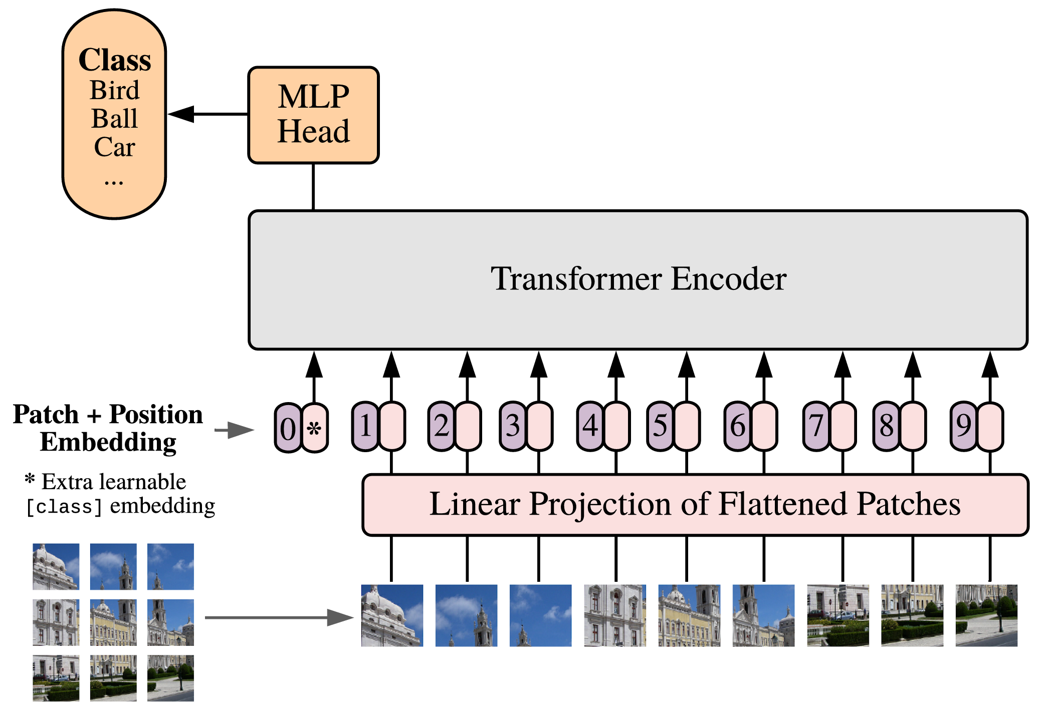
Given an image, ViT first cuts it into multiple patches; then it flattens each patch and maps it into a fixed-dimensional vector through a linear layer; next it adds positional encoding so that the model knows where each patch comes from; finally, it feeds these patch embeddings into a Transformer Encoder, using self-attention to model the relationships among different patches.
If the task is image classification, the model also needs to obtain a representation of the whole image. The original ViT does this by adding an extra class token. This token interacts with all patch tokens through multiple layers of self-attention, and its final output representation is used for classification. Of course, it is also possible to avoid using a class token and directly average-pool the outputs of all patch tokens.
So the core modules of ViT can be understood through the following questions:
- How does an image become a token sequence? Cut it into patches.
- How does each patch become a vector that Transformer can process? Use patch embedding.
- After flattening into a sequence, how does the model know the positions of the patches? Add positional embedding.
- How do we obtain a representation of the whole image? Add a class token or use average pooling.
- How do patches exchange information with each other? Use self-attention in the Transformer Encoder.
We can see that ViT is not simply a pile of modules. Each module is introduced to solve a concrete problem encountered when “feeding an image into Transformer.”
11.1.6 Core Differences Between CNN and ViT
When understanding ViT, a common misunderstanding is to simply regard it as replacing CNN with Transformer. This is not completely wrong, but it is too simple. More accurately, CNN and ViT make different assumptions about image structure.
| Model | Basic unit | Information interaction method | Main inductive bias |
|---|---|---|---|
| CNN | Pixel neighborhood / local feature | Local convolution gradually expands the receptive field layer by layer | Locality, parameter sharing, hierarchical structure |
| ViT | Image patch | Self-attention among patches | Weaker visual prior, more direct global interaction |
CNN’s way of modeling images depends more on visual priors. It assumes that local neighborhoods are important, that the same pattern can appear at different positions, and that complex semantics can be composed layer by layer from simple local features. These priors allow CNNs to train well even when the amount of data is not that large, because the model does not need to learn all image structures from scratch.
ViT has weaker priors. It does not directly require each patch to look only at nearby patches first, nor does it force the use of local convolution to expand the receptive field layer by layer. After cutting the image into a patch sequence, it lets self-attention learn how patches should interact. This is more flexible and easier to scale to large-scale data and large models, but it also means the model needs to learn more visual regularities from data.
This is also why the original ViT performs well on large-scale data, but is not necessarily naturally better than CNNs on smaller datasets. ViT’s advantages come from a more general sequence modeling approach and better scalability. But it also needs a large amount of data and appropriate training strategies to fully realize its potential.
11.1.7 Summary
In this section, we started from the way CNN models images and discussed the basic motivation of Vision Transformer.
CNNs are very suitable for images because they use visual priors such as locality, weight sharing, and hierarchical structure. They usually start by extracting features from local regions, and then gradually expand the receptive field through multiple stacked layers to integrate global information. Self-attention provides another idea: representations at different positions can interact directly, making it more flexible for modeling long-range relationships.
However, the input of Transformer is a token sequence, while an image is originally a two-dimensional grid. The key step of ViT is to cut the image into patches and treat each patch as a visual token. In this way, the image can be represented as a patch sequence and then processed by a Transformer Encoder.
Therefore, the core of ViT is not simply replacing CNN with Transformer, but first reorganizing the image into a sequence and then using self-attention to model the relationships among patches. Next, we will discuss the first step in detail: patch embedding. That is, how we convert patches in an image into token embeddings that Transformer can process.