import dnnlpy.nn as dnn
import torch
import torch.nn as nn
from torch import Tensor

print('PyTorch version:', torch.__version__)
PyTorch version: 2.13.0+cpu
In the previous section, we discussed the basic idea of Vision Transformer: since Transformer is good at processing sequences, can we also turn an image into a sequence and then let Transformer model it?
This idea sounds natural, but it immediately brings up a concrete problem: Transformer does not receive raw images, but a sequence of token embeddings. In natural language processing, the input is usually a sequence of tokens, and each token is mapped to an embedding; an image, however, is originally a two-dimensional grid and does not have ready-made tokens.
Therefore, the first step of ViT is not self-attention, but an input conversion first:
\[ \text{image} \quad \longrightarrow \quad \text{patch token sequence} \]
In this section, we focus only on this step, namely patch embedding. It answers the question:
How do we convert an image into a token embedding sequence that Transformer can process?
import dnnlpy.nn as dnn
import torch
import torch.nn as nn
from torch import Tensor
print('PyTorch version:', torch.__version__)PyTorch version: 2.13.0+cpuLet us first recall the input form of Transformer. For a sequence of length \(N\), the input can usually be written as:
\[ X = [x_1, x_2, \dots, x_N] \]
where each token embedding is a \(D\)-dimensional vector:
\[ x_i \in \mathbb{R}^{D} \]
If we use the batch-first format, the input tensor has shape:
\[ X \in \mathbb{R}^{B \times N \times D} \]
where \(B\) is the batch size, \(N\) is the sequence length, and \(D\) is the embedding dimension.
In other words, Transformer expects an input like this:
A group of tokens, where each token is a vector.But an image is usually:
\[ X \in \mathbb{R}^{B \times C \times H \times W} \]
where \(C\) is the number of channels, and \(H\) and \(W\) are the height and width of the image.
The meanings of these two tensors are completely different. An image is a two-dimensional spatial grid, with multiple color channels at each position; Transformer wants to see a one-dimensional token sequence, where each token is already a fixed-dimensional vector.
So what patch embedding needs to do can be summarized as:
\[ \mathbb{R}^{B \times C \times H \times W} \quad \longrightarrow \quad \mathbb{R}^{B \times N \times D} \]
Here, \(N\) is the number of tokens obtained after the image is cut into patches, and \(D\) is the embedding dimension used by Transformer.
In other words, patch embedding is the input translator of ViT. It translates an image from a two-dimensional grid in visual space into a token embedding sequence familiar to Transformer.
Now, let us formally introduce patch embedding. It is the first design in the input part of ViT, and also one of the most central designs.
We can divide patch embedding into two steps:
The first step is to cut the image into a group of non-overlapping small blocks. Suppose the input image size is \(H \times W\), and the patch size is \(P \times P\). For simplicity, assume first that both \(H\) and \(W\) are divisible by \(P\). Then there are \(\frac{H}{P}\) patches along the height dimension and \(\frac{W}{P}\) patches along the width dimension. So the total number of patches is:
\[ N = \frac{H}{P} \times \frac{W}{P} \]
The second step is to turn each patch into a vector. For an RGB image, the shape of a patch is:
\[ (C, P, P) \]
After flattening it, we obtain a vector of length \(C \times P^2\). Then we use a linear layer to project this vector to the embedding dimension \(D\) used by Transformer:
\[ C \times P^2 \rightarrow D \]
If we put the batch dimension and all patches together, the overall shape change of patch embedding is:
\[ (B, C, H, W) \rightarrow (B, N, C \times P^2) \rightarrow (B, N, D) \]
Each \(D\)-dimensional vector here is a patch token, or it can also be called a visual token.
For example, for a \(224 \times 224\) RGB image, if the patch size is \(16 \times 16\), then the patch grid size is:
\[ \frac{224}{16} \times \frac{224}{16} = 14 \times 14 \]
That is, one image is cut into 196 patches. Each patch is originally a small image block with shape \((3, 16, 16)\), and after flattening it becomes a \(3 \times 16 \times 16 = 768\)-dimensional vector.
If we also set the embedding dimension to \(D = 768\), then the output is:
\[ (B, 3, 224, 224) \rightarrow (B, 196, 768) \]
This is a very common setting in the original ViT (Dosovitskiy et al. 2021).
We first implement patchify in the most intuitive way, converting the image from the original input into patch embeddings. The goal here is not maximum efficiency, but to see clearly how the tensor shape changes.
Suppose the input image has shape \((B, C, H, W)\). We want to cut it into patches of size \(P \times P\) (assuming divisibility), and then flatten them into \((B, N, C P^2)\). Here, \(N\) is the number of patches, and \(C P^2\) is the flattened dimension of each patch.
def patchify(x: Tensor, patch_size: int) -> Tensor:
    batch_size, channels, height, width = x.size()
    if height % patch_size != 0 or width % patch_size != 0:
        raise AssertionError(
            'Image height and width must be divisible by `patch_size`.'
        )

    num_patches_h = height // patch_size
    num_patches_w = width // patch_size

    # (B, C, num_patches_h, W, patch_size)
    x = x.unfold(2, patch_size, patch_size)
    # (B, C, num_patches_h, num_patches_w, patch_size, patch_size)
    x = x.unfold(3, patch_size, patch_size)
    # (B, num_patches_h, num_patches_w, C, patch_size, patch_size)
    x = x.permute(0, 2, 3, 1, 4, 5)
    # NOTE: We can't use `view` here because the tensor is not
    # contiguous after `permute`.
    # (B, num_patches_h * num_patches_w, C * patch_size * patch_size)
    x = x.reshape(batch_size, num_patches_h * num_patches_w, -1)
    return x
Let us use a small example to look at the output shape:
patch_size = 8

x = torch.randn(2, 3, 32, 32)
patches = patchify(x, patch_size)

print('Input shape:', x.shape)
print('Patch shape:', patches.shape)
Input shape: torch.Size([2, 3, 32, 32])
Patch shape: torch.Size([2, 16, 192])In this example, the image size is \(32 \times 32\), and the patch size is \(8 \times 8\). So each image has
\[ \frac{32}{8} \times \frac{32}{8} = 4 \times 4 = 16 \]
patches, and the flattened dimension of each patch is
\[ 3 \times 8 \times 8 = 192 \]
Therefore, the final output shape is (2, 16, 192).
The parts most likely to cause confusion here are unfold and permute. We can understand them in three steps.
In the first step, use unfold to split the height and width separately. One part indicates “which patch this is,” and the other part indicates “which pixel inside the patch this is”:
\[ (B, C, H, W) \xrightarrow{\operatorname{unfold}(2, P, P)} \left(B, C, \frac{H}{P}, W, P\right) \xrightarrow{\operatorname{unfold}(3, P, P)} \left(B, C, \frac{H}{P}, \frac{W}{P}, P, P\right) \]
In the second step, use permute to adjust the dimension order. We want to first arrange patches according to their grid positions in the original image (that is, \(\frac{H}{P}\) and \(\frac{W}{P}\)), and then put the internal content of each patch afterward (that is, the channel dimension \(C\) and the internal \(P \times P\) spatial positions):
\[ \left(B, C, \frac{H}{P}, \frac{W}{P}, P, P\right) \rightarrow \left(B, \frac{H}{P}, \frac{W}{P}, C, P, P\right) \]
In the third step, flatten the two-dimensional patch grid into a one-dimensional sequence, and at the same time flatten the inside of each patch into a vector:
\[ \left(B, \frac{H}{P}, \frac{W}{P}, C, P, P\right) \rightarrow (B, N, C P^2) \]
In this way, we obtain a patch sequence.
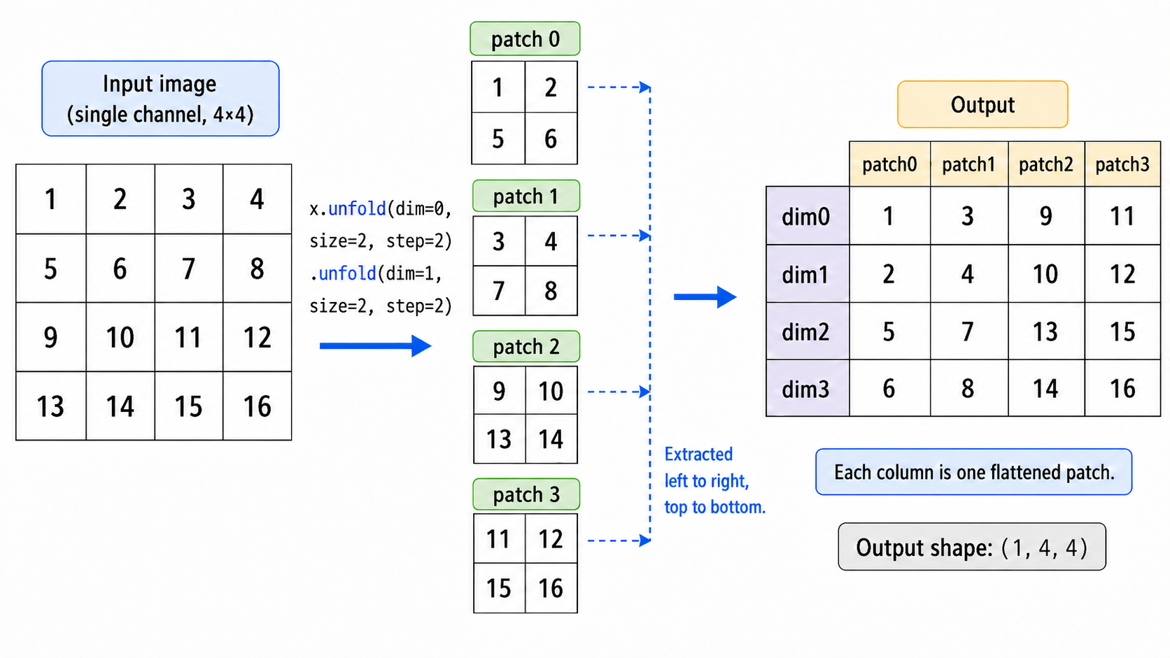
Tensor.unfold(dim, size, step) takes sliding windows along the dim dimension, where size is the window length and step is the window stride. Every time it obtains a window, it stacks that window, and the extra dimension indicates which window it is.
Compared with using Tensor.unfold twice, we can also directly use nn.Unfold(kernel_size=P, stride=P). It directly outputs a tensor of shape \((B, C P^2, N)\), and we only need to transpose the dimensions to obtain \((B, N, C P^2)\).
Linearpatchify only completes the first step:
\[ (B, C, H, W) \rightarrow (B, N, C P^2) \]
Next, we need to use a linear layer to project each patch vector to the embedding dimension \(D\):
\[ (B, N, C P^2) \rightarrow (B, N, D) \]
This is the most intuitive implementation of patch embedding.
class ViTLinearPatchEmbedding(nn.Module):
    def __init__(
        self,
        image_size: int = 224,
        patch_size: int = 16,
        in_channels: int = 3,
        embed_dim: int = 768,
    ):
        super().__init__()
        if image_size % patch_size != 0:
            raise AssertionError('`image_size` must be divisible by `patch_size`.')

        self.image_size = image_size
        self.patch_size = patch_size
        self.num_patches = (image_size // patch_size) ** 2
        self.proj = dnn.Linear(in_channels * patch_size * patch_size, embed_dim)

    def forward(self, x: Tensor) -> Tensor:
        patches = patchify(x, self.patch_size)
        embeddings = self.proj(patches)
        return embeddings
Test the output shape:
patch_embed = ViTLinearPatchEmbedding(
    image_size=32,
    patch_size=8,
    in_channels=3,
    embed_dim=64,
)

x = torch.randn(2, 3, 32, 32)
out = patch_embed(x)

print('Patch embedding output shape:', out.shape)
print('Number of patches:', patch_embed.num_patches)
Patch embedding output shape: torch.Size([2, 16, 64])
Number of patches: 16This shows that each image is cut into 16 patches, and each patch is mapped to a 64-dimensional token embedding.
At this point, the image has already become a sequence form that Transformer can receive:
\[ (B, C, H, W) \rightarrow (B, N, C P^2) \rightarrow (B, N, D) \]
Conv2dThe implementation above is very intuitive, but in actual ViT code, the more common way is to implement patch embedding with nn.Conv2d. This looks a little strange: isn’t ViT trying to move away from CNNs? Why is a convolution used again in the input layer?
The key is that the convolution here is not used to stack local feature extractors, but to efficiently complete:
\[ \text{patchify} + \text{linear projection} \]
If we use a convolution layer:
nn.Conv2d(
    in_channels=C,
    out_channels=D,
    kernel_size=P,
    stride=P,
)
then it slides a \(P \times P\) convolution kernel over the image with stride \(P\). Because kernel_size = stride = patch_size, these windows are exactly non-overlapping patches.
For each patch, the convolution layer maps the local region of shape \((C, P, P)\) to a \(D\)-dimensional output. This process is formally equivalent to “flattening a patch and then applying a linear layer”:
\[ \text{patchify} + \text{Linear} \quad \Longleftrightarrow \quad \operatorname{Conv2d}(\text{kernel\_size}=P, \text{stride}=P) \]
Below is the patch embedding implemented with Conv2d:
class ViTConvPatchEmbedding(nn.Module):
    def __init__(
        self,
        image_size: int = 224,
        patch_size: int = 16,
        in_channels: int = 3,
        embed_dim: int = 768,
    ):
        super().__init__()
        if image_size % patch_size != 0:
            raise AssertionError('`image_size` must be divisible by `patch_size`.')

        self.image_size = image_size
        self.patch_size = patch_size
        self.num_patches = (image_size // patch_size) ** 2

        self.proj = dnn.Conv2d(
            in_channels=in_channels,
            out_channels=embed_dim,
            kernel_size=patch_size,
            stride=patch_size,
        )

    def forward(self, x: Tensor) -> Tensor:
        x = self.proj(x)
        x = x.flatten(2)
        x = x.transpose(1, 2)
        return x
Test it:
patch_embed = ViTConvPatchEmbedding(
    image_size=32,
    patch_size=8,
    in_channels=3,
    embed_dim=64,
)

x = torch.randn(2, 3, 32, 32)
out = patch_embed(x)

print('Patch embedding output shape:', out.shape)
print('Number of patches:', patch_embed.num_patches)
Patch embedding output shape: torch.Size([2, 16, 64])
Number of patches: 16Here, the output shape of Conv2d is:
\[ \left(B, D, \frac{H}{P}, \frac{W}{P}\right) \]
This is still a two-dimensional feature map. To pass it to Transformer, we need to flatten the last two spatial dimensions into the sequence length:
x = x.flatten(2)  # (B, D, H/P * W/P)
x = x.transpose(1, 2)  # (B, N, D)
The final shape is still:
\[ (B, N, D) \]
So implementing patch embedding with Conv2d is just a more concise and more efficient engineering implementation. The convolution layer here is only responsible for cutting the image into patch tokens, rather than gradually extracting hierarchical features through multiple layers of local convolution like a CNN.
Linear and Conv2d Equivalent?We can understand the relationship between the Linear version and the Conv2d version more concretely.
For a patch, after flattening, it is a vector:
\[ x_i \in \mathbb{R}^{C P^2} \]
The weight of the linear layer is:
\[ W \in \mathbb{R}^{D \times C P^2} \]
The output is:
\[ z_i = W x_i + b \]
In Conv2d, each output channel has a convolution kernel of size \((C, P, P)\). If this convolution kernel is flattened, it is also a vector of length \(C P^2\). Applying convolution to a certain patch is essentially taking the inner product between this flattened convolution kernel and the patch vector. At the same time, because there are \(D\) output channels, this is equivalent to having \(D\) such linear projection directions. Putting them together is equivalent to a linear layer from \(C P^2\) to \(D\).
Therefore, Linear and Conv2d are mathematically equivalent. Both complete the conversion from the raw image to patch embeddings:
patchify + Linear matches the concept better and is suitable for teaching;Conv2d(kernel_size=P, stride=P) is more concise and closer to many real ViT implementations.Of course, we can also manually copy the weights of Linear into Conv2d to verify that their outputs are consistent. Interested readers can try it themselves.
In ViT, patch size is not just an implementation detail. It directly affects the computation cost and modeling behavior of ViT.
Assume the image size is fixed as \(H \times W\), and the patch size is \(P\). Then the sequence length is:
\[ N = \frac{H}{P} \times \frac{W}{P} \]
If \(P\) becomes smaller, the number of patches increases and the sequence becomes longer. Each token then covers a smaller local region, so more image details are preserved, but the computation and memory cost of self-attention also increase significantly. If \(P\) becomes larger, the number of patches decreases and the sequence becomes shorter. Computation becomes cheaper, but each token covers a larger region, and more fine-grained spatial information may be lost.
For example, for a \(224 \times 224\) image:
| Patch size | Patch grid | Sequence length \(N\) | Single-head Attention matrix size |
|---|---|---|---|
| \(8 \times 8\) | \(28 \times 28\) | \(784\) | About 2.35 MB |
| \(16 \times 16\) | \(14 \times 14\) | \(196\) | About 0.15 MB |
| \(32 \times 32\) | \(7 \times 7\) | \(49\) | About 0.009 MB |
The attention matrix size here is estimated by \(N \times N\) float32 elements. Since the attention matrix size is roughly proportional to \(N^2\), changing from \(16 \times 16\) patches to \(8 \times 8\) patches does not merely make the sequence length 4 times larger; it makes the attention matrix about 16 times larger. This is also why patch_size=16 is a common setting in the original ViT. It provides a fairly practical trade-off among sequence length, computation cost, and image detail.
Of course, patch size is not simply the smaller the better, nor the larger the better. It is related to data scale, model size, task type, and input resolution. For image classification, larger patches are sometimes already enough; for dense prediction tasks such as detection and segmentation, fine-grained spatial information is more important, so directly using a plain ViT architecture will encounter some difficulties. We will discuss these issues later when talking about visual Transformer variants.
In this section, we solved the first problem in the input part of ViT: how does an image become a token sequence that Transformer can receive?
Patch embedding does two things:
Therefore, it completes the following conversion:
\[ (B, C, H, W) \rightarrow (B, N, C P^2) \rightarrow (B, N, D) \]
In implementation, patch embedding can be completed in two ways. The first is to explicitly patchify and then apply Linear; the second is to use Conv2d(kernel_size=P, stride=P). The latter is mathematically equivalent to manually cutting patches plus linear projection, and it is also the more common way in actual implementations.
At this point, the image has already been translated into a sequence of patch tokens. But this is still not the complete input to the ViT Encoder.
There are two reasons. First, patch tokens only represent local image blocks. For image classification, we still need a global representation that can represent the whole image. Second, after patches are flattened into a one-dimensional sequence, the original two-dimensional spatial positions are weakened. Transformer sees a sequence of vectors, but it does not naturally know whether a patch comes from the upper-left corner, the center, or the lower-right corner.
So in the next section, we will add two designs: class token and positional embedding. The former solves the problem of “who represents the whole image,” and the latter solves the problem of “where each patch comes from.”