7.2 Dropout: Reducing Overfitting through Random Deactivation

Author

jshn9515

Published

2026-06-26

Modified

2026-06-26

In the previous section, we divided the common problems in deep networks into two categories: overfitting, which tends to occur when a model becomes too expressive, and optimization difficulties, which may arise as a network becomes deeper. Although Dropout and normalization are often used together, they address problems in different ways.

This section first discusses Dropout (Srivastava et al. 2014). Its operation looks straightforward: randomly set some intermediate activations to 0 during training. But this is not simply a matter of deleting some neurons. It continuously perturbs the network’s information paths during training, preventing the model from becoming overly dependent on a few fixed features.

Dropout also has an easily overlooked detail: why do the retained activations need to be divided by the keep probability? And why can dropout be turned off directly during inference after activations are randomly dropped during training? Once these questions are understood, dropout naturally becomes an operation that can be derived from probabilistic expectations.

import torch
import torch.nn as nn
import torch.nn.functional as F
from torch import Tensor

print('PyTorch version:', torch.__version__)

PyTorch version: 2.13.0+cpu

7.2.1 Why Can Randomly Dropping Activations Mitigate Overfitting?

Suppose a network contains many hidden units. When training lasts long enough, different hidden units may gradually form very fixed cooperation patterns. For example, a unit may be useful only when another unit is activated at the same time, or the classification result may depend heavily on a small number of features appearing together.

This phenomenon is usually called co-adaptation between features. Co-adaptation is not necessarily a problem by itself, but if a model relies too heavily on specific feature combinations in the training set, those combinations may no longer hold when the data distribution changes slightly, and the model’s generalization ability will decline.

Dropout works as follows: during each forward pass, it randomly disables some activations. As a result, a hidden unit cannot assume that the other units will always be present. To complete the task, the network must distribute information across more features and more paths instead of relying on one fragile, fixed combination.

For example, suppose a layer produces four features:

\[ x = [x_1, x_2, x_3, x_4] \]

Different forward passes may produce different masks:

forward 1: [1, 0, 1, 1]
forward 2: [0, 1, 1, 0]
forward 3: [1, 1, 0, 1]

Thus, every time the same sample passes through the network, the feature combination that actually participates in subsequent computations may be different. The model is no longer training one completely fixed information path, but many random subnetworks that share parameters.

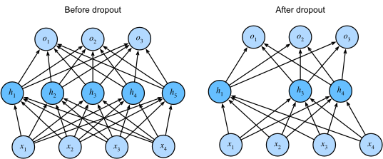
Figure 7.2.1 Dropout randomly selects subnetworks during training (Zhang et al. 2023, fig. 4.6.1)

From this perspective, Dropout adds structured noise to the training process. It usually makes the training task somewhat more difficult, so training loss may decrease more slowly and even training-set accuracy may be slightly lower. However, if the regularization strength is appropriate, validation-set performance may instead be better.

This is a typical characteristic of regularization methods:

They do not necessarily make it easier for a model to fit the training set; instead, they hope the model learns more robust patterns that can transfer to unseen examples.

7.2.2 The Mathematical Form of Dropout

Let the input activation be:

\[ x = [x_1, x_2, \dots, x_d] \]

For each element, we independently sample a Bernoulli random variable:

\[ m_i \sim \operatorname{Bernoulli}(1-p) \]

Here, \(p\) is the drop probability, and \(1-p\) is the keep probability. When \(m_i=0\), the \(i\)-th activation is dropped; when \(m_i=1\), the activation is retained. The most direct expression is:

\[ \tilde{x} = m \odot x \]

However, modern deep-learning frameworks usually use inverted dropout:

\[ \tilde{x} = \frac{m \odot x}{1-p} \]

In other words, during training, not only are some elements set to 0, but the retained elements are also multiplied by \(\tfrac{1}{1-p}\).

For example, when \(p=0.5\), approximately half of the activations are dropped and the remaining activations are multiplied by 2:

input:   [1, 2, 3, 4]
mask:    [1, 0, 1, 0]
output:  [2, 0, 6, 0]

The output values here look larger than the input values, but their overall expectation has not changed. This scaling is the key to allowing dropout to switch naturally between training and inference.

Let us first observe PyTorch’s behavior directly:

x = torch.ones(10)
output = F.dropout(x, p=0.5)

print('Input:')
print(x)
print('Dropout output:')
print(output)
print('Unique output values:', output.unique().tolist())

Input:
tensor([1., 1., 1., 1., 1., 1., 1., 1., 1., 1.])
Dropout output:
tensor([2., 0., 2., 0., 2., 2., 2., 2., 0., 2.])
Unique output values: [0.0, 2.0]

When the input consists entirely of 1s and p=0.5, the output usually contains only 0 and 2. 0 means that the element was dropped, while 2 means that the element was retained and divided by the keep probability \(1-p=0.5\).

7.2.3 Why Divide by the Keep Probability?

The most important detail of inverted dropout is this: why must the training-stage output be divided by \(1-p\)?

For an individual element \(x_i\), the dropout output is:

\[ \tilde{x}_i = \frac{m_i x_i}{1-p} \]

Because:

\[ \mathbb{E}[m_i] = 1-p \]

we have:

\[ \begin{align} \mathbb{E}[\tilde{x}_i] &= \mathbb{E}\left[\frac{m_i x_i}{1-p}\right] \\ &= \frac{x_i}{1-p}\mathbb{E}[m_i] \\ &= \frac{x_i}{1-p}(1-p) \\ &= x_i \end{align} \]

Therefore, although a single forward pass randomly changes the output, under a large number of random samples the expected value of the dropout output is still equal to the original input.

We repeatedly apply dropout to the same tensor and then calculate the mean of all outputs:

x = torch.tensor([1.0, 2.0, 3.0, 4.0])
outputs = torch.stack([F.dropout(x, p=0.5) for _ in range(10000)])

print('Original input:', x)
print('Mean dropout output:', outputs.mean(dim=0))

Original input: tensor([1., 2., 3., 4.])
Mean dropout output: tensor([1.0110, 1.9992, 2.9862, 3.9968])

As the number of samples increases, the mean output gradually approaches the original input.

If training computes only \(m \odot x\) without scaling the retained activation values, then because each neuron has a probability of only \(1-p\) of being retained, the expected output during training is:

\[ \mathbb{E}[m \odot x] = (1-p) \cdot x \]

During inference, dropout is disabled, all neurons participate in the computation, and the output returns to \(x\). This creates an inconsistency in activation scale between training and inference: the training expectation is \((1-p) \cdot x\), while the inference output is \(x\).

One way to solve this is to multiply the output by \(1-p\) during inference so that it matches training. Inverted dropout uses a more convenient approach: during training, divide the retained activation values by \(1-p\). In this way, the expected output during training remains \(x\). During inference, we only need to turn off dropout and do not need any additional scaling.

That is:

\[ \begin{align} \text{training:} &\quad \tilde{x}=\frac{m\odot x}{1-p} \\ \text{inference:} &\quad \tilde{x}=x \end{align} \]

This is also the implementation typically used by frameworks such as PyTorch and TensorFlow.

Note that what is preserved is the expectation of the output, not the numerical value of every output or its variance. Dropout increases the randomness and variance of activations during training, which is part of the reason it can serve as a regularizer.

7.2.4 A PyTorch Implementation of Dropout

After understanding the mask and scaling, we can implement a minimal version of dropout ourselves. We need to handle three cases:

Return the input directly in inference mode;
Drop no elements when p=0;
Sample a mask and divide by the keep probability in training mode.

def dropout(
    x: Tensor,
    p: float = 0.5,
    training: bool = True,
) -> Tensor:
    """Randomly zero elements of the input tensor."""
    if not 0.0 <= p <= 1.0:
        raise AssertionError(f'`p` must be between 0 and 1, but got {p}.')

    if not training or p == 0.0:
        return x

    if p == 1.0:
        return torch.zeros_like(x)

    keep = 1.0 - p
    mask = torch.rand_like(x) < keep
    return x * mask / keep

We can compare this implementation with F.dropout:

x = torch.arange(10, dtype=torch.float32)

actual = dropout(x, p=0.25)
expected = F.dropout(x, p=0.25)

print('Custom dropout:', actual, sep='\n')
print('PyTorch dropout:', expected, sep='\n')

Custom dropout:
tensor([ 0.0000,  0.0000,  2.6667,  4.0000,  5.3333,  6.6667,  0.0000,  9.3333,
        10.6667, 12.0000])
PyTorch dropout:
tensor([ 0.0000,  0.0000,  0.0000,  4.0000,  0.0000,  0.0000,  0.0000,  9.3333,
        10.6667, 12.0000])

The two implementations will not necessarily produce exactly the same mask because their underlying random-sampling processes may differ, but they should have the same statistical behavior: each element is set to 0 with probability \(p\), and each retained element is multiplied by \(\tfrac{1}{1-p}\).

Next, we wrap it in an nn.Module:

class Dropout(nn.Module):
    """Randomly zero elements of the input tensor."""

    def __init__(self, p: float = 0.5):
        super().__init__()
        if not 0.0 <= p <= 1.0:
            raise AssertionError(f'`p` must be between 0 and 1, but got {p}.')
        self.p = p

    def forward(self, x: Tensor) -> Tensor:
        return dropout(x, p=self.p, training=self.training)

    def extra_repr(self) -> str:
        return f'p={self.p}'

The most noteworthy detail here is self.training. Every nn.Module maintains a training state: when model.train() is called, self.training=True; when model.eval() is called, self.training=False. Dropout uses this state to decide whether to sample a random mask.

7.2.5 Training Mode and Inference Mode

Dropout should be enabled only during training. During inference, we want the model to use all features and produce deterministic output for the same input.

dropout = nn.Dropout(p=0.5)
x = torch.ones(10)

dropout.train()
train_output1 = dropout(x)
train_output2 = dropout(x)

dropout.eval()
eval_output1 = dropout(x)
eval_output2 = dropout(x)

print('Training output 1:', train_output1)
print('Training output 2:', train_output2)
print('Evaluation output 1:', eval_output1)
print('Evaluation output 2:', eval_output2)

Training output 1: tensor([0., 0., 0., 0., 2., 0., 2., 0., 0., 0.])
Training output 2: tensor([0., 0., 2., 2., 0., 2., 2., 0., 0., 2.])
Evaluation output 1: tensor([1., 1., 1., 1., 1., 1., 1., 1., 1., 1.])
Evaluation output 2: tensor([1., 1., 1., 1., 1., 1., 1., 1., 1., 1.])

In training mode, the two outputs are usually different because a new mask is sampled each time. In inference mode, dropout returns the input directly, so the two outputs are exactly the same.

This also shows that torch.no_grad() or torch.inference_mode() does not automatically turn off dropout. These contexts control whether autograd records a computation graph, whereas whether dropout is active is determined by the module’s training state. For example:

dropout = nn.Dropout(p=0.5)
dropout.train()

with torch.inference_mode():
    x = torch.ones(8)
    y = dropout(x)

print(y)

tensor([2., 2., 0., 2., 2., 2., 2., 0.])

Even in inference_mode(), as long as the module remains in training mode, dropout will still randomly drop elements.

Therefore, standard inference code usually contains both:

model = nn.Sequential(
    nn.Linear(4, 8),
    nn.ReLU(),
    nn.Dropout(p=0.5),
    nn.Linear(8, 2),
)

model.eval()
x = torch.randn(3, 4)

with torch.inference_mode():
    y = model(x)

print('y.shape:', y.shape)

y.shape: torch.Size([3, 2])

model.eval() switches the behavior of modules such as Dropout and BatchNorm, while torch.inference_mode() disables gradient recording. They serve different purposes and cannot replace each other.

7.2.6 What Does Dropout Do During Backpropagation?

Dropout changes not only the activations in the forward pass, but also the gradient paths in backpropagation.

For:

\[ \tilde{x}_i = \frac{m_i x_i}{1-p} \]

the local gradient is:

\[ \frac{\partial \tilde{x}_i}{\partial x_i} = \frac{m_i}{1-p} \]

Therefore:

For a dropped element, \(m_i=0\), so its gradient is also 0;
For a retained element, \(m_i=1\), so its gradient is multiplied by \(\tfrac{1}{1-p}\).

In other words, an information path that is disabled during one forward pass will likewise receive no gradient during the corresponding backward pass.

We can check this directly:

x = torch.ones(12, requires_grad=True)
y = F.dropout(x, p=0.5)
y.backward(gradient=torch.ones_like(y))

print('Dropout output:', y.data)
print('Input gradient:', x.grad)

Dropout output: tensor([0., 0., 2., 0., 0., 0., 0., 2., 0., 2., 0., 0.])
Input gradient: tensor([0., 0., 2., 0., 0., 0., 0., 2., 0., 2., 0., 0.])

Because the input consists entirely of 1s and the loss is the sum of all outputs, the output and input gradient usually have the same mask: at dropped positions, both the output and gradient are 0; at retained positions, both the output and gradient are 2.

At the same time, dropout does not separately modify gradients after backward(). It first changes the computation graph in the forward pass, after which autograd naturally differentiates through this random computation graph. This differs from gradient clipping. Gradient clipping explicitly modifies the .grad attribute of parameters after backward() has computed the gradients, whereas dropout is part of the network’s forward computation.

7.2.7 `nn.Dropout` and `F.dropout`

PyTorch provides the module form nn.Dropout and the function form F.dropout. They perform the same operation but suit different scenarios.

With nn.Dropout, the drop probability and training state are managed by the module:

class MLP1(nn.Module):
    def __init__(self, input_dim: int, output_dim: int):
        super().__init__()
        self.layers = nn.Sequential(
            nn.Linear(input_dim, 256),
            nn.ReLU(),
            nn.Dropout(p=0.2),
            nn.Linear(256, output_dim),
        )

    def forward(self, x: Tensor) -> Tensor:
        return self.layers(x)

With the function form, you need to pass training=self.training explicitly:

class MLP2(nn.Module):
    def __init__(self, input_dim: int, output_dim: int):
        super().__init__()
        self.fc1 = nn.Linear(input_dim, 256)
        self.fc2 = nn.Linear(256, output_dim)

    def forward(self, x: Tensor) -> Tensor:
        x = self.fc1(x)
        x = F.relu(x)
        x = F.dropout(x, p=0.2, training=self.training)
        x = self.fc2(x)
        return x

Here, training=self.training cannot be omitted. The default value of the training parameter in F.dropout is True. If you write:

x = F.dropout(x, p=0.2)

then even if the outer model has already called model.eval(), the function may continue to perform dropout.

Therefore, in ordinary network architectures, using nn.Dropout is usually less error-prone. The function form is more convenient only when the drop probability needs to change dynamically or when dropout is just one part of a custom computation.

7.2.8 Dropout1d, Dropout2d, and Dropout3d

nn.Dropout independently samples a mask for every element in the input. However, adjacent spatial positions in convolutional feature maps are usually highly correlated. Dropping only a few individual pixel positions may leave very similar information in the remaining positions, so the regularization effect may be weak.

Therefore, PyTorch also provides:

nn.Dropout1d;
nn.Dropout2d;
nn.Dropout3d.

These do not mean that the input must separately be a one-, two-, or three-dimensional tensor. Here, 1d/2d/3d refers to the spatial dimensions of convolutional features, and their core behavior is:

Randomly drop entire channels instead of independently dropping every element.

For a two-dimensional convolutional output:

\[ X \in \mathbb{R}^{N \times C \times H \times W} \]

nn.Dropout2d samples one mask for each sample and channel, and then sets the selected entire \(H\times W\) feature map to 0:

\[ \tilde{X}_{n,c,:,:} = 0 \]

Below, we compare ordinary Dropout and Dropout2d:

x = torch.ones(1, 4, 3, 3)

element_dropout = nn.Dropout(p=0.5)
channel_dropout = nn.Dropout2d(p=0.5)

element_output = element_dropout(x)
channel_output = channel_dropout(x)

print('Element-wise dropout:')
print(element_output)

print('\nChannel-wise dropout:')
print(channel_output)

Element-wise dropout:
tensor([[[[2., 0., 0.],
          [2., 2., 2.],
          [0., 2., 2.]],

         [[2., 0., 2.],
          [0., 2., 2.],
          [2., 2., 2.]],

         [[2., 2., 2.],
          [0., 2., 2.],
          [0., 2., 2.]],

         [[2., 2., 2.],
          [0., 2., 2.],
          [0., 0., 2.]]]])

Channel-wise dropout:
tensor([[[[0., 0., 0.],
          [0., 0., 0.],
          [0., 0., 0.]],

         [[0., 0., 0.],
          [0., 0., 0.],
          [0., 0., 0.]],

         [[0., 0., 0.],
          [0., 0., 0.],
          [0., 0., 0.]],

         [[0., 0., 0.],
          [0., 0., 0.],
          [0., 0., 0.]]]])

Ordinary Dropout produces scattered 0s within each feature map. Dropout2d, on the other hand, turns some channels entirely into 0 while retaining and scaling the other channels as a whole.

These modules can be roughly understood as follows:

Table 7.2.8 Typical Inputs for Different Dropout Modules in PyTorch
Module	Typical input	Unit randomly dropped
`nn.Dropout`	Any shape	Individual element
`nn.Dropout1d`	\((N,C,L)\)	Entire one-dimensional channel
`nn.Dropout2d`	\((N,C,H,W)\)	Entire two-dimensional channel
`nn.Dropout3d`	\((N,C,D,H,W)\)	Entire three-dimensional channel

Therefore, Dropout2d is not ordinary dropout applied to a two-dimensional matrix, but channel-wise dropout for two-dimensional convolutional feature maps. Dropout1d and Dropout3d work analogously. Their goal is to randomly disable some channels in convolutional feature maps, thereby reducing co-adaptation between features.

7.2.9 Where Should Dropout Be Placed?

Dropout is usually placed where there are many learnable parameters and where overfitting is more likely, such as in MLP hidden layers or classification heads:

Linear → Activation → Dropout → Linear

The corresponding code can be written as:

block = nn.Sequential(
    nn.Linear(128, 256),
    nn.ReLU(),
    nn.Dropout(p=0.2),
    nn.Linear(256, 10),
)

In Transformers, dropout may appear in multiple places, such as attention weights, attention outputs, feed-forward networks, and residual branches. However, the specific placement is part of the model architecture design, which we will discuss in detail later in the chapters related to Transformers.

For CNNs, traditional models sometimes use channel-wise dropout in convolutional blocks and often use ordinary dropout in the fully connected layer of the final classifier. However, whether modern CNNs need dropout should be considered together with data augmentation, weight decay, BatchNorm, and model size.

At the same time, the dropout probability is not better when it is larger:

If \(p\) is too small, the regularization effect may be insignificant;
If \(p\) is too large, too much information is lost and the model may underfit;
The smaller the network and the more abundant the data, the less strong dropout is usually needed;
The more prone the model is to overfitting, the more reason there is to increase dropout.

A common value of \(p\) may lie between 0.1 and 0.5. Whether to use dropout and what probability to use should be determined based on validation-set performance.

7.2.10 Common Misconceptions about Dropout

To avoid mixing dropout up with other training techniques, let us clarify several common misconceptions.

First, dropout is not normalization. It does not compute means and variances, nor does it actively adjust activations to a fixed scale. Dividing by \(1-p\) is only for preserving the expectation, not for implementing standardization.

Second, dropout is not model pruning. Although some activations are temporarily set to 0 during training, the dropped positions may be different each time, and the parameters themselves remain. The complete network is usually still used during inference. Pruning permanently removes weights, connections, or channels, and its usual goal is to reduce model size or computational cost.

Third, dropout is not gradient clipping. Dropout randomly changes the computation path during the forward pass; gradient clipping limits the gradient magnitude after backpropagation is complete. Their points of application are entirely different.

Finally, more dropout is not always better. It is a regularization method, and it is valuable only when the model is at risk of overfitting. If the model is already underfitting, increasing dropout further will only weaken its capacity.

The core content of this section can be summarized as follows:

Table 7.2.10 Core Properties of Dropout
Question	Conclusion
What problem does dropout mainly solve?	Mitigate overfitting through random perturbations
What does it do during training?	Randomly zero activations and divide retained values by \(1-p\)
Why is scaling needed?	Keep the output expectation consistent with the input
What does it do during inference?	Turn off dropout and use the complete activations directly
Does it modify model parameters?	No; it only temporarily changes the activation and gradient paths
What does `Dropout2d` drop?	Entire two-dimensional feature channels rather than individual pixels

7.2.11 Summary

Dropout is a stochastic regularization method that acts on intermediate activations. During training, it samples a random mask for each element or channel and temporarily disables some information paths, thereby reducing the model’s overreliance on fixed feature combinations.

PyTorch uses inverted dropout:

\[ \tilde{x} = \frac{m\odot x}{1-p} \]

After dividing by the keep probability, the expected output during training is consistent with the original input. Therefore, during inference, we only need to turn off dropout and do not need additional scaling.

The training and inference behavior of dropout is controlled by the training attribute. model.eval() can turn off dropout, whereas torch.no_grad() and torch.inference_mode() are responsible only for disabling gradient recording and cannot replace eval().

Ordinary nn.Dropout independently drops elements, whereas nn.Dropout{n}d usually drops entire channels at a time. They suit convolutional features with different shapes, but their common goal is to reduce co-adaptation between features through random perturbations.

In the next section, we begin discussing Batch Normalization (Ioffe and Szegedy 2015). Unlike dropout, BatchNorm does not randomly disable features; instead, it adjusts the numerical scale of activations according to mini-batch statistics. We will focus on answering the following questions: for fully connected inputs and convolutional inputs, over which dimensions does BatchNorm actually compute the mean and variance, and why does it use different statistics during training and inference?

References

Ioffe, Sergey, and Christian Szegedy. 2015. Batch Normalization: Accelerating Deep Network Training by Reducing Internal Covariate Shift. https://arxiv.org/abs/1502.03167.

Srivastava, Nitish, Geoffrey Hinton, Alex Krizhevsky, Ilya Sutskever, and Ruslan Salakhutdinov. 2014. “Dropout: A Simple Way to Prevent Neural Networks from Overfitting.” Journal of Machine Learning Research 15 (56): 1929–58. http://jmlr.org/papers/v15/srivastava14a.html.

Zhang, Aston, Zachary C. Lipton, Mu Li, and Alexander J. Smola. 2023. Dive into Deep Learning. Cambridge University Press. https://D2L.ai.

Reuse

CC BY-NC 4.0